Tall Arrays
Calculate with arrays that have more rows than fit in memory.
This function fully supports tall arrays. For
more information, see Tall Arrays.
C/C++ Code Generation
Generate C and C++ code using MATLAB® Coder™.
Usage notes and limitations:
-
Strict single-precision calculations are not supported. In the generated code,
single-precision inputs produce single-precision outputs. However, variables inside the
function might be double-precision.
Thread-Based Environment
Run code in the background using MATLAB® backgroundPool or accelerate code with Parallel Computing Toolbox™ ThreadPool.
GPU Arrays
Accelerate code by running on a graphics processing unit (GPU) using Parallel Computing Toolbox™.
This function fully supports GPU arrays. For more information, see Run MATLAB Functions on a GPU (Parallel Computing Toolbox).
Distributed Arrays
Partition large arrays across the combined memory of your cluster using Parallel Computing Toolbox™.
«Высокие» массивы
Осуществление вычислений с массивами, которые содержат больше строк, чем помещается в памяти.
Генерация кода C/C++
Генерация кода C и C++ с помощью MATLAB® Coder™.
Указания и ограничения по применению:
-
Строгие вычисления с одинарной точностью не поддерживаются. В сгенерированном коде входные параметры с одинарной точностью производят выходные параметры с одинарной точностью. Однако переменные в функциональной силе быть с двойной точностью.
Основанная на потоке среда
Запустите код в фоновом режиме с помощью MATLAB® backgroundPool или ускорьте код с Parallel Computing Toolbox™ ThreadPool.
Массивы графического процессора
Ускорьте код путем работы графического процессора (GPU) с помощью Parallel Computing Toolbox™.
Эта функция полностью поддерживает массивы графического процессора. Для получения дополнительной информации смотрите функции MATLAB Запуска на графическом процессоре (Parallel Computing Toolbox).
Распределенные массивы
Большие массивы раздела через объединенную память о вашем кластере с помощью Parallel Computing Toolbox™.
| Error function | |
|---|---|
Plot of the error function |
|
| General information | |
| General definition |  |
| Fields of application | Probability, thermodynamics |
| Domain, Codomain and Image | |
| Domain |  |
| Image |  |
| Basic features | |
| Parity | Odd |
| Specific features | |
| Root | 0 |
| Derivative |  |
| Antiderivative |  |
| Series definition | |
| Taylor series |  |
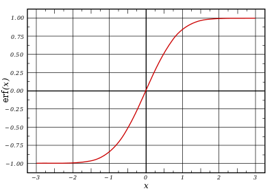
In mathematics, the error function (also called the Gauss error function), often denoted by erf, is a complex function of a complex variable defined as:[1]

This integral is a special (non-elementary) sigmoid function that occurs often in probability, statistics, and partial differential equations. In many of these applications, the function argument is a real number. If the function argument is real, then the function value is also real.
In statistics, for non-negative values of x, the error function has the following interpretation: for a random variable Y that is normally distributed with mean 0 and standard deviation 1/√2, erf x is the probability that Y falls in the range [−x, x].
Two closely related functions are the complementary error function (erfc) defined as

and the imaginary error function (erfi) defined as

where i is the imaginary unit
Name[edit]
The name «error function» and its abbreviation erf were proposed by J. W. L. Glaisher in 1871 on account of its connection with «the theory of Probability, and notably the theory of Errors.»[2] The error function complement was also discussed by Glaisher in a separate publication in the same year.[3]
For the «law of facility» of errors whose density is given by

(the normal distribution), Glaisher calculates the probability of an error lying between p and q as:
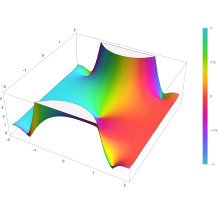
Plot of the error function Erf(z) in the complex plane from -2-2i to 2+2i with colors created with Mathematica 13.1 function ComplexPlot3D

Applications[edit]
When the results of a series of measurements are described by a normal distribution with standard deviation σ and expected value 0, then erf (a/σ √2) is the probability that the error of a single measurement lies between −a and +a, for positive a. This is useful, for example, in determining the bit error rate of a digital communication system.
The error and complementary error functions occur, for example, in solutions of the heat equation when boundary conditions are given by the Heaviside step function.
The error function and its approximations can be used to estimate results that hold with high probability or with low probability. Given a random variable X ~ Norm[μ,σ] (a normal distribution with mean μ and standard deviation σ) and a constant L < μ:
![{displaystyle {begin{aligned}Pr[Xleq L]&={frac {1}{2}}+{frac {1}{2}}operatorname {erf} {frac {L-mu }{{sqrt {2}}sigma }}&approx Aexp left(-Bleft({frac {L-mu }{sigma }}right)^{2}right)end{aligned}}}](https://wikimedia.org/api/rest_v1/media/math/render/svg/f3cb760eaf336393db9fd0bb12c4465655a27de8)
where A and B are certain numeric constants. If L is sufficiently far from the mean, specifically μ − L ≥ σ√ln k, then:
![{displaystyle Pr[Xleq L]leq Aexp(-Bln {k})={frac {A}{k^{B}}}}](https://wikimedia.org/api/rest_v1/media/math/render/svg/2baadea015e20a45d1034fd88eed861e7fcce178)
so the probability goes to 0 as k → ∞.
The probability for X being in the interval [La, Lb] can be derived as
![{displaystyle {begin{aligned}Pr[L_{a}leq Xleq L_{b}]&=int _{L_{a}}^{L_{b}}{frac {1}{{sqrt {2pi }}sigma }}exp left(-{frac {(x-mu )^{2}}{2sigma ^{2}}}right),mathrm {d} x&={frac {1}{2}}left(operatorname {erf} {frac {L_{b}-mu }{{sqrt {2}}sigma }}-operatorname {erf} {frac {L_{a}-mu }{{sqrt {2}}sigma }}right).end{aligned}}}](https://wikimedia.org/api/rest_v1/media/math/render/svg/cd2214f0db2c1d36075815825b616501175c6283)
Properties[edit]
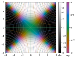
Integrand exp(−z2)

erf z
The property erf (−z) = −erf z means that the error function is an odd function. This directly results from the fact that the integrand e−t2 is an even function (the antiderivative of an even function which is zero at the origin is an odd function and vice versa).
Since the error function is an entire function which takes real numbers to real numbers, for any complex number z:

where z is the complex conjugate of z.
The integrand f = exp(−z2) and f = erf z are shown in the complex z-plane in the figures at right with domain coloring.
The error function at +∞ is exactly 1 (see Gaussian integral). At the real axis, erf z approaches unity at z → +∞ and −1 at z → −∞. At the imaginary axis, it tends to ±i∞.
Taylor series[edit]
The error function is an entire function; it has no singularities (except that at infinity) and its Taylor expansion always converges, but is famously known «[…] for its bad convergence if x > 1.»[4]
The defining integral cannot be evaluated in closed form in terms of elementary functions, but by expanding the integrand e−z2 into its Maclaurin series and integrating term by term, one obtains the error function’s Maclaurin series as:
![{displaystyle {begin{aligned}operatorname {erf} z&={frac {2}{sqrt {pi }}}sum _{n=0}^{infty }{frac {(-1)^{n}z^{2n+1}}{n!(2n+1)}}[6pt]&={frac {2}{sqrt {pi }}}left(z-{frac {z^{3}}{3}}+{frac {z^{5}}{10}}-{frac {z^{7}}{42}}+{frac {z^{9}}{216}}-cdots right)end{aligned}}}](https://wikimedia.org/api/rest_v1/media/math/render/svg/c80541f305af070bb0510625c584fe1559a0cd2c)
which holds for every complex number z. The denominator terms are sequence A007680 in the OEIS.
For iterative calculation of the above series, the following alternative formulation may be useful:
![{displaystyle {begin{aligned}operatorname {erf} z&={frac {2}{sqrt {pi }}}sum _{n=0}^{infty }left(zprod _{k=1}^{n}{frac {-(2k-1)z^{2}}{k(2k+1)}}right)[6pt]&={frac {2}{sqrt {pi }}}sum _{n=0}^{infty }{frac {z}{2n+1}}prod _{k=1}^{n}{frac {-z^{2}}{k}}end{aligned}}}](https://wikimedia.org/api/rest_v1/media/math/render/svg/dca22e8e7dee0297e87a455249c282c6b92fedcb)
because −(2k − 1)z2/k(2k + 1) expresses the multiplier to turn the kth term into the (k + 1)th term (considering z as the first term).
The imaginary error function has a very similar Maclaurin series, which is:
![{displaystyle {begin{aligned}operatorname {erfi} z&={frac {2}{sqrt {pi }}}sum _{n=0}^{infty }{frac {z^{2n+1}}{n!(2n+1)}}[6pt]&={frac {2}{sqrt {pi }}}left(z+{frac {z^{3}}{3}}+{frac {z^{5}}{10}}+{frac {z^{7}}{42}}+{frac {z^{9}}{216}}+cdots right)end{aligned}}}](https://wikimedia.org/api/rest_v1/media/math/render/svg/2ff91095cd6825137cc951ec0a786db0b7f68fac)
which holds for every complex number z.
Derivative and integral[edit]
The derivative of the error function follows immediately from its definition:

From this, the derivative of the imaginary error function is also immediate:

An antiderivative of the error function, obtainable by integration by parts, is

An antiderivative of the imaginary error function, also obtainable by integration by parts, is

Higher order derivatives are given by

where H are the physicists’ Hermite polynomials.[5]
Bürmann series[edit]
An expansion,[6] which converges more rapidly for all real values of x than a Taylor expansion, is obtained by using Hans Heinrich Bürmann’s theorem:[7]
![{displaystyle {begin{aligned}operatorname {erf} x&={frac {2}{sqrt {pi }}}operatorname {sgn} xcdot {sqrt {1-e^{-x^{2}}}}left(1-{frac {1}{12}}left(1-e^{-x^{2}}right)-{frac {7}{480}}left(1-e^{-x^{2}}right)^{2}-{frac {5}{896}}left(1-e^{-x^{2}}right)^{3}-{frac {787}{276480}}left(1-e^{-x^{2}}right)^{4}-cdots right)[10pt]&={frac {2}{sqrt {pi }}}operatorname {sgn} xcdot {sqrt {1-e^{-x^{2}}}}left({frac {sqrt {pi }}{2}}+sum _{k=1}^{infty }c_{k}e^{-kx^{2}}right).end{aligned}}}](https://wikimedia.org/api/rest_v1/media/math/render/svg/164e7f029977edb47c83845b04abfe5b2d28b837)
where sgn is the sign function. By keeping only the first two coefficients and choosing c1 = 31/200 and c2 = −341/8000, the resulting approximation shows its largest relative error at x = ±1.3796, where it is less than 0.0036127:

Inverse functions[edit]
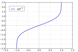
Given a complex number z, there is not a unique complex number w satisfying erf w = z, so a true inverse function would be multivalued. However, for −1 < x < 1, there is a unique real number denoted erf−1 x satisfying

The inverse error function is usually defined with domain (−1,1), and it is restricted to this domain in many computer algebra systems. However, it can be extended to the disk |z| < 1 of the complex plane, using the Maclaurin series

where c0 = 1 and

So we have the series expansion (common factors have been canceled from numerators and denominators):

(After cancellation the numerator/denominator fractions are entries OEIS: A092676/OEIS: A092677 in the OEIS; without cancellation the numerator terms are given in entry OEIS: A002067.) The error function’s value at ±∞ is equal to ±1.
For |z| < 1, we have erf(erf−1 z) = z.
The inverse complementary error function is defined as

For real x, there is a unique real number erfi−1 x satisfying erfi(erfi−1 x) = x. The inverse imaginary error function is defined as erfi−1 x.[8]
For any real x, Newton’s method can be used to compute erfi−1 x, and for −1 ≤ x ≤ 1, the following Maclaurin series converges:

where ck is defined as above.
Asymptotic expansion[edit]
A useful asymptotic expansion of the complementary error function (and therefore also of the error function) for large real x is
![{displaystyle {begin{aligned}operatorname {erfc} x&={frac {e^{-x^{2}}}{x{sqrt {pi }}}}left(1+sum _{n=1}^{infty }(-1)^{n}{frac {1cdot 3cdot 5cdots (2n-1)}{left(2x^{2}right)^{n}}}right)[6pt]&={frac {e^{-x^{2}}}{x{sqrt {pi }}}}sum _{n=0}^{infty }(-1)^{n}{frac {(2n-1)!!}{left(2x^{2}right)^{n}}},end{aligned}}}](https://wikimedia.org/api/rest_v1/media/math/render/svg/35a11e2e5b22ca898c74f2e913d276c9ac11124a)
where (2n − 1)!! is the double factorial of (2n − 1), which is the product of all odd numbers up to (2n − 1). This series diverges for every finite x, and its meaning as asymptotic expansion is that for any integer N ≥ 1 one has

where the remainder, in Landau notation, is

as x → ∞.
Indeed, the exact value of the remainder is

which follows easily by induction, writing

and integrating by parts.
For large enough values of x, only the first few terms of this asymptotic expansion are needed to obtain a good approximation of erfc x (while for not too large values of x, the above Taylor expansion at 0 provides a very fast convergence).
Continued fraction expansion[edit]
A continued fraction expansion of the complementary error function is:[9]

Integral of error function with Gaussian density function[edit]

which appears related to Ng and Geller, formula 13 in section 4.3[10] with a change of variables.
Factorial series[edit]
The inverse factorial series:

converges for Re(z2) > 0. Here

zn denotes the rising factorial, and s(n,k) denotes a signed Stirling number of the first kind.[11][12]
There also exists a representation by an infinite sum containing the double factorial:

Numerical approximations[edit]
Approximation with elementary functions[edit]
- Abramowitz and Stegun give several approximations of varying accuracy (equations 7.1.25–28). This allows one to choose the fastest approximation suitable for a given application. In order of increasing accuracy, they are:
(maximum error: 5×10⁻⁴)
where a1 = 0.278393, a2 = 0.230389, a3 = 0.000972, a4 = 0.078108
(maximum error: 2.5×10⁻⁵)
where p = 0.47047, a1 = 0.3480242, a2 = −0.0958798, a3 = 0.7478556
(maximum error: 3×10⁻⁷)
where a1 = 0.0705230784, a2 = 0.0422820123, a3 = 0.0092705272, a4 = 0.0001520143, a5 = 0.0002765672, a6 = 0.0000430638
(maximum error: 1.5×10⁻⁷)
where p = 0.3275911, a1 = 0.254829592, a2 = −0.284496736, a3 = 1.421413741, a4 = −1.453152027, a5 = 1.061405429
All of these approximations are valid for x ≥ 0. To use these approximations for negative x, use the fact that erf x is an odd function, so erf x = −erf(−x).
- Exponential bounds and a pure exponential approximation for the complementary error function are given by[13]
- The above have been generalized to sums of N exponentials[14] with increasing accuracy in terms of N so that erfc x can be accurately approximated or bounded by 2Q̃(√2x), where
In particular, there is a systematic methodology to solve the numerical coefficients {(an,bn)}N
n = 1 that yield a minimax approximation or bound for the closely related Q-function: Q(x) ≈ Q̃(x), Q(x) ≤ Q̃(x), or Q(x) ≥ Q̃(x) for x ≥ 0. The coefficients {(an,bn)}N
n = 1 for many variations of the exponential approximations and bounds up to N = 25 have been released to open access as a comprehensive dataset.[15] - A tight approximation of the complementary error function for x ∈ [0,∞) is given by Karagiannidis & Lioumpas (2007)[16] who showed for the appropriate choice of parameters {A,B} that
They determined {A,B} = {1.98,1.135}, which gave a good approximation for all x ≥ 0. Alternative coefficients are also available for tailoring accuracy for a specific application or transforming the expression into a tight bound.[17]
- A single-term lower bound is[18]
where the parameter β can be picked to minimize error on the desired interval of approximation.
-
- Another approximation is given by Sergei Winitzki using his «global Padé approximations»:[19][20]: 2–3
where
This is designed to be very accurate in a neighborhood of 0 and a neighborhood of infinity, and the relative error is less than 0.00035 for all real x. Using the alternate value a ≈ 0.147 reduces the maximum relative error to about 0.00013.[21]
This approximation can be inverted to obtain an approximation for the inverse error function:
- An approximation with a maximal error of 1.2×10⁻⁷ for any real argument is:[22]
with
and


Table of values[edit]
| x | erf x | 1 − erf x |
|---|---|---|
| 0 | 0 | 1 |
| 0.02 | 0.022564575 | 0.977435425 |
| 0.04 | 0.045111106 | 0.954888894 |
| 0.06 | 0.067621594 | 0.932378406 |
| 0.08 | 0.090078126 | 0.909921874 |
| 0.1 | 0.112462916 | 0.887537084 |
| 0.2 | 0.222702589 | 0.777297411 |
| 0.3 | 0.328626759 | 0.671373241 |
| 0.4 | 0.428392355 | 0.571607645 |
| 0.5 | 0.520499878 | 0.479500122 |
| 0.6 | 0.603856091 | 0.396143909 |
| 0.7 | 0.677801194 | 0.322198806 |
| 0.8 | 0.742100965 | 0.257899035 |
| 0.9 | 0.796908212 | 0.203091788 |
| 1 | 0.842700793 | 0.157299207 |
| 1.1 | 0.880205070 | 0.119794930 |
| 1.2 | 0.910313978 | 0.089686022 |
| 1.3 | 0.934007945 | 0.065992055 |
| 1.4 | 0.952285120 | 0.047714880 |
| 1.5 | 0.966105146 | 0.033894854 |
| 1.6 | 0.976348383 | 0.023651617 |
| 1.7 | 0.983790459 | 0.016209541 |
| 1.8 | 0.989090502 | 0.010909498 |
| 1.9 | 0.992790429 | 0.007209571 |
| 2 | 0.995322265 | 0.004677735 |
| 2.1 | 0.997020533 | 0.002979467 |
| 2.2 | 0.998137154 | 0.001862846 |
| 2.3 | 0.998856823 | 0.001143177 |
| 2.4 | 0.999311486 | 0.000688514 |
| 2.5 | 0.999593048 | 0.000406952 |
| 3 | 0.999977910 | 0.000022090 |
| 3.5 | 0.999999257 | 0.000000743 |
[edit]
Complementary error function[edit]
The complementary error function, denoted erfc, is defined as
-
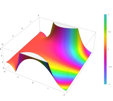
Plot of the complementary error function Erfc(z) in the complex plane from -2-2i to 2+2i with colors created with Mathematica 13.1 function ComplexPlot3D
![{displaystyle {begin{aligned}operatorname {erfc} x&=1-operatorname {erf} x[5pt]&={frac {2}{sqrt {pi }}}int _{x}^{infty }e^{-t^{2}},mathrm {d} t[5pt]&=e^{-x^{2}}operatorname {erfcx} x,end{aligned}}}](https://wikimedia.org/api/rest_v1/media/math/render/svg/4acd0062271e2a19c209a02c8cc33d44a28af7cc)
which also defines erfcx, the scaled complementary error function[23] (which can be used instead of erfc to avoid arithmetic underflow[23][24]). Another form of erfc x for x ≥ 0 is known as Craig’s formula, after its discoverer:[25]

This expression is valid only for positive values of x, but it can be used in conjunction with erfc x = 2 − erfc(−x) to obtain erfc(x) for negative values. This form is advantageous in that the range of integration is fixed and finite. An extension of this expression for the erfc of the sum of two non-negative variables is as follows:[26]

Imaginary error function[edit]
The imaginary error function, denoted erfi, is defined as

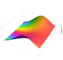
Plot of the imaginary error function Erfi(z) in the complex plane from -2-2i to 2+2i with colors created with Mathematica 13.1 function ComplexPlot3D
![{displaystyle {begin{aligned}operatorname {erfi} x&=-ioperatorname {erf} ix[5pt]&={frac {2}{sqrt {pi }}}int _{0}^{x}e^{t^{2}},mathrm {d} t[5pt]&={frac {2}{sqrt {pi }}}e^{x^{2}}D(x),end{aligned}}}](https://wikimedia.org/api/rest_v1/media/math/render/svg/bfd2dd94cd6d0325224d412f6b5e5ed63ca81d4a)
where D(x) is the Dawson function (which can be used instead of erfi to avoid arithmetic overflow[23]).
Despite the name «imaginary error function», erfi x is real when x is real.
When the error function is evaluated for arbitrary complex arguments z, the resulting complex error function is usually discussed in scaled form as the Faddeeva function:

Cumulative distribution function[edit]
The error function is essentially identical to the standard normal cumulative distribution function, denoted Φ, also named norm(x) by some software languages[citation needed], as they differ only by scaling and translation. Indeed,
-
the normal cumulative distribution function plotted in the complex plane
![{displaystyle {begin{aligned}Phi (x)&={frac {1}{sqrt {2pi }}}int _{-infty }^{x}e^{tfrac {-t^{2}}{2}},mathrm {d} t[6pt]&={frac {1}{2}}left(1+operatorname {erf} {frac {x}{sqrt {2}}}right)[6pt]&={frac {1}{2}}operatorname {erfc} left(-{frac {x}{sqrt {2}}}right)end{aligned}}}](https://wikimedia.org/api/rest_v1/media/math/render/svg/89a9e9eaaddcd7a91ade15a41b8d1e272d437559)
or rearranged for erf and erfc:
![{displaystyle {begin{aligned}operatorname {erf} (x)&=2Phi left(x{sqrt {2}}right)-1[6pt]operatorname {erfc} (x)&=2Phi left(-x{sqrt {2}}right)&=2left(1-Phi left(x{sqrt {2}}right)right).end{aligned}}}](https://wikimedia.org/api/rest_v1/media/math/render/svg/86c84a4d2d79631fe9996e30f1d6c0da3089bfe2)
Consequently, the error function is also closely related to the Q-function, which is the tail probability of the standard normal distribution. The Q-function can be expressed in terms of the error function as

The inverse of Φ is known as the normal quantile function, or probit function and may be expressed in terms of the inverse error function as

The standard normal cdf is used more often in probability and statistics, and the error function is used more often in other branches of mathematics.
The error function is a special case of the Mittag-Leffler function, and can also be expressed as a confluent hypergeometric function (Kummer’s function):

It has a simple expression in terms of the Fresnel integral.[further explanation needed]
In terms of the regularized gamma function P and the incomplete gamma function,

sgn x is the sign function.
Generalized error functions[edit]

Graph of generalised error functions En(x):
grey curve: E1(x) = 1 − e−x/√π
red curve: E2(x) = erf(x)
green curve: E3(x)
blue curve: E4(x)
gold curve: E5(x).
Some authors discuss the more general functions:[citation needed]

Notable cases are:
- E0(x) is a straight line through the origin: E0(x) = x/e√π
- E2(x) is the error function, erf x.
After division by n!, all the En for odd n look similar (but not identical) to each other. Similarly, the En for even n look similar (but not identical) to each other after a simple division by n!. All generalised error functions for n > 0 look similar on the positive x side of the graph.
These generalised functions can equivalently be expressed for x > 0 using the gamma function and incomplete gamma function:

Therefore, we can define the error function in terms of the incomplete gamma function:

Iterated integrals of the complementary error function[edit]
The iterated integrals of the complementary error function are defined by[27]
![{displaystyle {begin{aligned}operatorname {i} ^{n}!operatorname {erfc} z&=int _{z}^{infty }operatorname {i} ^{n-1}!operatorname {erfc} zeta ,mathrm {d} zeta [6pt]operatorname {i} ^{0}!operatorname {erfc} z&=operatorname {erfc} zoperatorname {i} ^{1}!operatorname {erfc} z&=operatorname {ierfc} z={frac {1}{sqrt {pi }}}e^{-z^{2}}-zoperatorname {erfc} zoperatorname {i} ^{2}!operatorname {erfc} z&={tfrac {1}{4}}left(operatorname {erfc} z-2zoperatorname {ierfc} zright)end{aligned}}}](https://wikimedia.org/api/rest_v1/media/math/render/svg/c3e7b953efaa4d730a5479bd61a2c378c8f761dc)
The general recurrence formula is

They have the power series

from which follow the symmetry properties

and

Implementations[edit]
As real function of a real argument[edit]
- In Posix-compliant operating systems, the header
math.hshall declare and the mathematical librarylibmshall provide the functionserfanderfc(double precision) as well as their single precision and extended precision counterpartserff,erflanderfcf,erfcl.[28] - The GNU Scientific Library provides
erf,erfc,log(erf), and scaled error functions.[29]
As complex function of a complex argument[edit]
libcerf, numeric C library for complex error functions, provides the complex functionscerf,cerfc,cerfcxand the real functionserfi,erfcxwith approximately 13–14 digits precision, based on the Faddeeva function as implemented in the MIT Faddeeva Package
See also[edit]
[edit]
- Gaussian integral, over the whole real line
- Gaussian function, derivative
- Dawson function, renormalized imaginary error function
- Goodwin–Staton integral
In probability[edit]
- Normal distribution
- Normal cumulative distribution function, a scaled and shifted form of error function
- Probit, the inverse or quantile function of the normal CDF
- Q-function, the tail probability of the normal distribution
References[edit]
- ^ Andrews, Larry C. (1998). Special functions of mathematics for engineers. SPIE Press. p. 110. ISBN 9780819426161.
- ^ Glaisher, James Whitbread Lee (July 1871). «On a class of definite integrals». London, Edinburgh, and Dublin Philosophical Magazine and Journal of Science. 4. 42 (277): 294–302. doi:10.1080/14786447108640568. Retrieved 6 December 2017.
- ^ Glaisher, James Whitbread Lee (September 1871). «On a class of definite integrals. Part II». London, Edinburgh, and Dublin Philosophical Magazine and Journal of Science. 4. 42 (279): 421–436. doi:10.1080/14786447108640600. Retrieved 6 December 2017.
- ^ «A007680 – OEIS». oeis.org. Retrieved 2 April 2020.
- ^ Weisstein, Eric W. «Erf». MathWorld.
- ^ Schöpf, H. M.; Supancic, P. H. (2014). «On Bürmann’s Theorem and Its Application to Problems of Linear and Nonlinear Heat Transfer and Diffusion». The Mathematica Journal. 16. doi:10.3888/tmj.16-11.
- ^ Weisstein, Eric W. «Bürmann’s Theorem». MathWorld.
- ^ Bergsma, Wicher (2006). «On a new correlation coefficient, its orthogonal decomposition and associated tests of independence». arXiv:math/0604627.
- ^ Cuyt, Annie A. M.; Petersen, Vigdis B.; Verdonk, Brigitte; Waadeland, Haakon; Jones, William B. (2008). Handbook of Continued Fractions for Special Functions. Springer-Verlag. ISBN 978-1-4020-6948-2.
- ^ Ng, Edward W.; Geller, Murray (January 1969). «A table of integrals of the Error functions». Journal of Research of the National Bureau of Standards Section B. 73B (1): 1. doi:10.6028/jres.073B.001.
- ^ Schlömilch, Oskar Xavier (1859). «Ueber facultätenreihen». Zeitschrift für Mathematik und Physik (in German). 4: 390–415. Retrieved 4 December 2017.
- ^ Nielson, Niels (1906). Handbuch der Theorie der Gammafunktion (in German). Leipzig: B. G. Teubner. p. 283 Eq. 3. Retrieved 4 December 2017.
- ^ Chiani, M.; Dardari, D.; Simon, M.K. (2003). «New Exponential Bounds and Approximations for the Computation of Error Probability in Fading Channels» (PDF). IEEE Transactions on Wireless Communications. 2 (4): 840–845. CiteSeerX 10.1.1.190.6761. doi:10.1109/TWC.2003.814350.
- ^ Tanash, I.M.; Riihonen, T. (2020). «Global minimax approximations and bounds for the Gaussian Q-function by sums of exponentials». IEEE Transactions on Communications. 68 (10): 6514–6524. arXiv:2007.06939. doi:10.1109/TCOMM.2020.3006902. S2CID 220514754.
- ^ Tanash, I.M.; Riihonen, T. (2020). «Coefficients for Global Minimax Approximations and Bounds for the Gaussian Q-Function by Sums of Exponentials [Data set]». Zenodo. doi:10.5281/zenodo.4112978.
- ^ Karagiannidis, G. K.; Lioumpas, A. S. (2007). «An improved approximation for the Gaussian Q-function» (PDF). IEEE Communications Letters. 11 (8): 644–646. doi:10.1109/LCOMM.2007.070470. S2CID 4043576.
- ^ Tanash, I.M.; Riihonen, T. (2021). «Improved coefficients for the Karagiannidis–Lioumpas approximations and bounds to the Gaussian Q-function». IEEE Communications Letters. 25 (5): 1468–1471. arXiv:2101.07631. doi:10.1109/LCOMM.2021.3052257. S2CID 231639206.
- ^ Chang, Seok-Ho; Cosman, Pamela C.; Milstein, Laurence B. (November 2011). «Chernoff-Type Bounds for the Gaussian Error Function». IEEE Transactions on Communications. 59 (11): 2939–2944. doi:10.1109/TCOMM.2011.072011.100049. S2CID 13636638.
- ^ Winitzki, Sergei (2003). «Uniform approximations for transcendental functions». Computational Science and Its Applications – ICCSA 2003. Lecture Notes in Computer Science. Vol. 2667. Springer, Berlin. pp. 780–789. doi:10.1007/3-540-44839-X_82. ISBN 978-3-540-40155-1.
- ^ Zeng, Caibin; Chen, Yang Cuan (2015). «Global Padé approximations of the generalized Mittag-Leffler function and its inverse». Fractional Calculus and Applied Analysis. 18 (6): 1492–1506. arXiv:1310.5592. doi:10.1515/fca-2015-0086. S2CID 118148950.
Indeed, Winitzki [32] provided the so-called global Padé approximation
- ^ Winitzki, Sergei (6 February 2008). «A handy approximation for the error function and its inverse».
- ^ Numerical Recipes in Fortran 77: The Art of Scientific Computing (ISBN 0-521-43064-X), 1992, page 214, Cambridge University Press.
- ^ a b c Cody, W. J. (March 1993), «Algorithm 715: SPECFUN—A portable FORTRAN package of special function routines and test drivers» (PDF), ACM Trans. Math. Softw., 19 (1): 22–32, CiteSeerX 10.1.1.643.4394, doi:10.1145/151271.151273, S2CID 5621105
- ^ Zaghloul, M. R. (1 March 2007), «On the calculation of the Voigt line profile: a single proper integral with a damped sine integrand», Monthly Notices of the Royal Astronomical Society, 375 (3): 1043–1048, Bibcode:2007MNRAS.375.1043Z, doi:10.1111/j.1365-2966.2006.11377.x
- ^ John W. Craig, A new, simple and exact result for calculating the probability of error for two-dimensional signal constellations Archived 3 April 2012 at the Wayback Machine, Proceedings of the 1991 IEEE Military Communication Conference, vol. 2, pp. 571–575.
- ^ Behnad, Aydin (2020). «A Novel Extension to Craig’s Q-Function Formula and Its Application in Dual-Branch EGC Performance Analysis». IEEE Transactions on Communications. 68 (7): 4117–4125. doi:10.1109/TCOMM.2020.2986209. S2CID 216500014.
- ^ Carslaw, H. S.; Jaeger, J. C. (1959), Conduction of Heat in Solids (2nd ed.), Oxford University Press, ISBN 978-0-19-853368-9, p 484
- ^ https://pubs.opengroup.org/onlinepubs/9699919799/basedefs/math.h.html
- ^ «Special Functions – GSL 2.7 documentation».
Further reading[edit]
- Abramowitz, Milton; Stegun, Irene Ann, eds. (1983) [June 1964]. «Chapter 7». Handbook of Mathematical Functions with Formulas, Graphs, and Mathematical Tables. Applied Mathematics Series. Vol. 55 (Ninth reprint with additional corrections of tenth original printing with corrections (December 1972); first ed.). Washington D.C.; New York: United States Department of Commerce, National Bureau of Standards; Dover Publications. p. 297. ISBN 978-0-486-61272-0. LCCN 64-60036. MR 0167642. LCCN 65-12253.
- Press, William H.; Teukolsky, Saul A.; Vetterling, William T.; Flannery, Brian P. (2007), «Section 6.2. Incomplete Gamma Function and Error Function», Numerical Recipes: The Art of Scientific Computing (3rd ed.), New York: Cambridge University Press, ISBN 978-0-521-88068-8
- Temme, Nico M. (2010), «Error Functions, Dawson’s and Fresnel Integrals», in Olver, Frank W. J.; Lozier, Daniel M.; Boisvert, Ronald F.; Clark, Charles W. (eds.), NIST Handbook of Mathematical Functions, Cambridge University Press, ISBN 978-0-521-19225-5, MR 2723248
External links[edit]
- A Table of Integrals of the Error Functions
| Error function | |
|---|---|
|
Plot of the error function |
|
| General information | |
| General definition | |
| Fields of application | Probability, thermodynamics |
| Domain, Codomain and Image | |
| Domain | |
| Image | |
| Basic features | |
| Parity | Odd |
| Specific features | |
| Root | 0 |
| Derivative | |
| Antiderivative | |
| Series definition | |
| Taylor series | |
In mathematics, the error function (also called the Gauss error function), often denoted by erf, is a complex function of a complex variable defined as:[1]
This integral is a special (non-elementary) sigmoid function that occurs often in probability, statistics, and partial differential equations. In many of these applications, the function argument is a real number. If the function argument is real, then the function value is also real.
In statistics, for non-negative values of x, the error function has the following interpretation: for a random variable Y that is normally distributed with mean 0 and standard deviation 1/√2, erf x is the probability that Y falls in the range [−x, x].
Two closely related functions are the complementary error function (erfc) defined as
and the imaginary error function (erfi) defined as
where i is the imaginary unit
Name[edit]
The name «error function» and its abbreviation erf were proposed by J. W. L. Glaisher in 1871 on account of its connection with «the theory of Probability, and notably the theory of Errors.»[2] The error function complement was also discussed by Glaisher in a separate publication in the same year.[3]
For the «law of facility» of errors whose density is given by
(the normal distribution), Glaisher calculates the probability of an error lying between p and q as:
Plot of the error function Erf(z) in the complex plane from -2-2i to 2+2i with colors created with Mathematica 13.1 function ComplexPlot3D
Applications[edit]
When the results of a series of measurements are described by a normal distribution with standard deviation σ and expected value 0, then erf (a/σ √2) is the probability that the error of a single measurement lies between −a and +a, for positive a. This is useful, for example, in determining the bit error rate of a digital communication system.
The error and complementary error functions occur, for example, in solutions of the heat equation when boundary conditions are given by the Heaviside step function.
The error function and its approximations can be used to estimate results that hold with high probability or with low probability. Given a random variable X ~ Norm[μ,σ] (a normal distribution with mean μ and standard deviation σ) and a constant L < μ:
where A and B are certain numeric constants. If L is sufficiently far from the mean, specifically μ − L ≥ σ√ln k, then:
so the probability goes to 0 as k → ∞.
The probability for X being in the interval [La, Lb] can be derived as
Properties[edit]
Integrand exp(−z2)
erf z
The property erf (−z) = −erf z means that the error function is an odd function. This directly results from the fact that the integrand e−t2 is an even function (the antiderivative of an even function which is zero at the origin is an odd function and vice versa).
Since the error function is an entire function which takes real numbers to real numbers, for any complex number z:
where z is the complex conjugate of z.
The integrand f = exp(−z2) and f = erf z are shown in the complex z-plane in the figures at right with domain coloring.
The error function at +∞ is exactly 1 (see Gaussian integral). At the real axis, erf z approaches unity at z → +∞ and −1 at z → −∞. At the imaginary axis, it tends to ±i∞.
Taylor series[edit]
The error function is an entire function; it has no singularities (except that at infinity) and its Taylor expansion always converges, but is famously known «[…] for its bad convergence if x > 1.»[4]
The defining integral cannot be evaluated in closed form in terms of elementary functions, but by expanding the integrand e−z2 into its Maclaurin series and integrating term by term, one obtains the error function’s Maclaurin series as:
which holds for every complex number z. The denominator terms are sequence A007680 in the OEIS.
For iterative calculation of the above series, the following alternative formulation may be useful:
because −(2k − 1)z2/k(2k + 1) expresses the multiplier to turn the kth term into the (k + 1)th term (considering z as the first term).
The imaginary error function has a very similar Maclaurin series, which is:
which holds for every complex number z.
Derivative and integral[edit]
The derivative of the error function follows immediately from its definition:
From this, the derivative of the imaginary error function is also immediate:
An antiderivative of the error function, obtainable by integration by parts, is
An antiderivative of the imaginary error function, also obtainable by integration by parts, is
Higher order derivatives are given by
where H are the physicists’ Hermite polynomials.[5]
Bürmann series[edit]
An expansion,[6] which converges more rapidly for all real values of x than a Taylor expansion, is obtained by using Hans Heinrich Bürmann’s theorem:[7]
where sgn is the sign function. By keeping only the first two coefficients and choosing c1 = 31/200 and c2 = −341/8000, the resulting approximation shows its largest relative error at x = ±1.3796, where it is less than 0.0036127:
Inverse functions[edit]
Given a complex number z, there is not a unique complex number w satisfying erf w = z, so a true inverse function would be multivalued. However, for −1 < x < 1, there is a unique real number denoted erf−1 x satisfying
The inverse error function is usually defined with domain (−1,1), and it is restricted to this domain in many computer algebra systems. However, it can be extended to the disk |z| < 1 of the complex plane, using the Maclaurin series
where c0 = 1 and
So we have the series expansion (common factors have been canceled from numerators and denominators):
(After cancellation the numerator/denominator fractions are entries OEIS: A092676/OEIS: A092677 in the OEIS; without cancellation the numerator terms are given in entry OEIS: A002067.) The error function’s value at ±∞ is equal to ±1.
For |z| < 1, we have erf(erf−1 z) = z.
The inverse complementary error function is defined as
For real x, there is a unique real number erfi−1 x satisfying erfi(erfi−1 x) = x. The inverse imaginary error function is defined as erfi−1 x.[8]
For any real x, Newton’s method can be used to compute erfi−1 x, and for −1 ≤ x ≤ 1, the following Maclaurin series converges:
where ck is defined as above.
Asymptotic expansion[edit]
A useful asymptotic expansion of the complementary error function (and therefore also of the error function) for large real x is
where (2n − 1)!! is the double factorial of (2n − 1), which is the product of all odd numbers up to (2n − 1). This series diverges for every finite x, and its meaning as asymptotic expansion is that for any integer N ≥ 1 one has
where the remainder, in Landau notation, is
as x → ∞.
Indeed, the exact value of the remainder is
which follows easily by induction, writing
and integrating by parts.
For large enough values of x, only the first few terms of this asymptotic expansion are needed to obtain a good approximation of erfc x (while for not too large values of x, the above Taylor expansion at 0 provides a very fast convergence).
Continued fraction expansion[edit]
A continued fraction expansion of the complementary error function is:[9]
Integral of error function with Gaussian density function[edit]
which appears related to Ng and Geller, formula 13 in section 4.3[10] with a change of variables.
Factorial series[edit]
The inverse factorial series:
converges for Re(z2) > 0. Here
zn denotes the rising factorial, and s(n,k) denotes a signed Stirling number of the first kind.[11][12]
There also exists a representation by an infinite sum containing the double factorial:
Numerical approximations[edit]
Approximation with elementary functions[edit]
- Abramowitz and Stegun give several approximations of varying accuracy (equations 7.1.25–28). This allows one to choose the fastest approximation suitable for a given application. In order of increasing accuracy, they are:
(maximum error: 5×10⁻⁴)
where a1 = 0.278393, a2 = 0.230389, a3 = 0.000972, a4 = 0.078108
(maximum error: 2.5×10⁻⁵)
where p = 0.47047, a1 = 0.3480242, a2 = −0.0958798, a3 = 0.7478556
(maximum error: 3×10⁻⁷)
where a1 = 0.0705230784, a2 = 0.0422820123, a3 = 0.0092705272, a4 = 0.0001520143, a5 = 0.0002765672, a6 = 0.0000430638
(maximum error: 1.5×10⁻⁷)
where p = 0.3275911, a1 = 0.254829592, a2 = −0.284496736, a3 = 1.421413741, a4 = −1.453152027, a5 = 1.061405429
All of these approximations are valid for x ≥ 0. To use these approximations for negative x, use the fact that erf x is an odd function, so erf x = −erf(−x).
- Exponential bounds and a pure exponential approximation for the complementary error function are given by[13]
- The above have been generalized to sums of N exponentials[14] with increasing accuracy in terms of N so that erfc x can be accurately approximated or bounded by 2Q̃(√2x), where
In particular, there is a systematic methodology to solve the numerical coefficients {(an,bn)}N
n = 1 that yield a minimax approximation or bound for the closely related Q-function: Q(x) ≈ Q̃(x), Q(x) ≤ Q̃(x), or Q(x) ≥ Q̃(x) for x ≥ 0. The coefficients {(an,bn)}N
n = 1 for many variations of the exponential approximations and bounds up to N = 25 have been released to open access as a comprehensive dataset.[15] - A tight approximation of the complementary error function for x ∈ [0,∞) is given by Karagiannidis & Lioumpas (2007)[16] who showed for the appropriate choice of parameters {A,B} that
They determined {A,B} = {1.98,1.135}, which gave a good approximation for all x ≥ 0. Alternative coefficients are also available for tailoring accuracy for a specific application or transforming the expression into a tight bound.[17]
- A single-term lower bound is[18]
where the parameter β can be picked to minimize error on the desired interval of approximation.
-
- Another approximation is given by Sergei Winitzki using his «global Padé approximations»:[19][20]: 2–3
where
This is designed to be very accurate in a neighborhood of 0 and a neighborhood of infinity, and the relative error is less than 0.00035 for all real x. Using the alternate value a ≈ 0.147 reduces the maximum relative error to about 0.00013.[21]
This approximation can be inverted to obtain an approximation for the inverse error function:
- An approximation with a maximal error of 1.2×10⁻⁷ for any real argument is:[22]
with
and
Table of values[edit]
| x | erf x | 1 − erf x |
|---|---|---|
| 0 | 0 | 1 |
| 0.02 | 0.022564575 | 0.977435425 |
| 0.04 | 0.045111106 | 0.954888894 |
| 0.06 | 0.067621594 | 0.932378406 |
| 0.08 | 0.090078126 | 0.909921874 |
| 0.1 | 0.112462916 | 0.887537084 |
| 0.2 | 0.222702589 | 0.777297411 |
| 0.3 | 0.328626759 | 0.671373241 |
| 0.4 | 0.428392355 | 0.571607645 |
| 0.5 | 0.520499878 | 0.479500122 |
| 0.6 | 0.603856091 | 0.396143909 |
| 0.7 | 0.677801194 | 0.322198806 |
| 0.8 | 0.742100965 | 0.257899035 |
| 0.9 | 0.796908212 | 0.203091788 |
| 1 | 0.842700793 | 0.157299207 |
| 1.1 | 0.880205070 | 0.119794930 |
| 1.2 | 0.910313978 | 0.089686022 |
| 1.3 | 0.934007945 | 0.065992055 |
| 1.4 | 0.952285120 | 0.047714880 |
| 1.5 | 0.966105146 | 0.033894854 |
| 1.6 | 0.976348383 | 0.023651617 |
| 1.7 | 0.983790459 | 0.016209541 |
| 1.8 | 0.989090502 | 0.010909498 |
| 1.9 | 0.992790429 | 0.007209571 |
| 2 | 0.995322265 | 0.004677735 |
| 2.1 | 0.997020533 | 0.002979467 |
| 2.2 | 0.998137154 | 0.001862846 |
| 2.3 | 0.998856823 | 0.001143177 |
| 2.4 | 0.999311486 | 0.000688514 |
| 2.5 | 0.999593048 | 0.000406952 |
| 3 | 0.999977910 | 0.000022090 |
| 3.5 | 0.999999257 | 0.000000743 |
[edit]
Complementary error function[edit]
The complementary error function, denoted erfc, is defined as
-
Plot of the complementary error function Erfc(z) in the complex plane from -2-2i to 2+2i with colors created with Mathematica 13.1 function ComplexPlot3D
which also defines erfcx, the scaled complementary error function[23] (which can be used instead of erfc to avoid arithmetic underflow[23][24]). Another form of erfc x for x ≥ 0 is known as Craig’s formula, after its discoverer:[25]
This expression is valid only for positive values of x, but it can be used in conjunction with erfc x = 2 − erfc(−x) to obtain erfc(x) for negative values. This form is advantageous in that the range of integration is fixed and finite. An extension of this expression for the erfc of the sum of two non-negative variables is as follows:[26]
Imaginary error function[edit]
The imaginary error function, denoted erfi, is defined as
Plot of the imaginary error function Erfi(z) in the complex plane from -2-2i to 2+2i with colors created with Mathematica 13.1 function ComplexPlot3D
where D(x) is the Dawson function (which can be used instead of erfi to avoid arithmetic overflow[23]).
Despite the name «imaginary error function», erfi x is real when x is real.
When the error function is evaluated for arbitrary complex arguments z, the resulting complex error function is usually discussed in scaled form as the Faddeeva function:
Cumulative distribution function[edit]
The error function is essentially identical to the standard normal cumulative distribution function, denoted Φ, also named norm(x) by some software languages[citation needed], as they differ only by scaling and translation. Indeed,
-
the normal cumulative distribution function plotted in the complex plane
or rearranged for erf and erfc:
Consequently, the error function is also closely related to the Q-function, which is the tail probability of the standard normal distribution. The Q-function can be expressed in terms of the error function as
The inverse of Φ is known as the normal quantile function, or probit function and may be expressed in terms of the inverse error function as
The standard normal cdf is used more often in probability and statistics, and the error function is used more often in other branches of mathematics.
The error function is a special case of the Mittag-Leffler function, and can also be expressed as a confluent hypergeometric function (Kummer’s function):
It has a simple expression in terms of the Fresnel integral.[further explanation needed]
In terms of the regularized gamma function P and the incomplete gamma function,
sgn x is the sign function.
Generalized error functions[edit]
Graph of generalised error functions En(x):
grey curve: E1(x) = 1 − e−x/√π
red curve: E2(x) = erf(x)
green curve: E3(x)
blue curve: E4(x)
gold curve: E5(x).
Some authors discuss the more general functions:[citation needed]
Notable cases are:
- E0(x) is a straight line through the origin: E0(x) = x/e√π
- E2(x) is the error function, erf x.
After division by n!, all the En for odd n look similar (but not identical) to each other. Similarly, the En for even n look similar (but not identical) to each other after a simple division by n!. All generalised error functions for n > 0 look similar on the positive x side of the graph.
These generalised functions can equivalently be expressed for x > 0 using the gamma function and incomplete gamma function:
Therefore, we can define the error function in terms of the incomplete gamma function:
Iterated integrals of the complementary error function[edit]
The iterated integrals of the complementary error function are defined by[27]
The general recurrence formula is
They have the power series
from which follow the symmetry properties
and
Implementations[edit]
As real function of a real argument[edit]
- In Posix-compliant operating systems, the header
math.hshall declare and the mathematical librarylibmshall provide the functionserfanderfc(double precision) as well as their single precision and extended precision counterpartserff,erflanderfcf,erfcl.[28] - The GNU Scientific Library provides
erf,erfc,log(erf), and scaled error functions.[29]
As complex function of a complex argument[edit]
libcerf, numeric C library for complex error functions, provides the complex functionscerf,cerfc,cerfcxand the real functionserfi,erfcxwith approximately 13–14 digits precision, based on the Faddeeva function as implemented in the MIT Faddeeva Package
See also[edit]
[edit]
- Gaussian integral, over the whole real line
- Gaussian function, derivative
- Dawson function, renormalized imaginary error function
- Goodwin–Staton integral
In probability[edit]
- Normal distribution
- Normal cumulative distribution function, a scaled and shifted form of error function
- Probit, the inverse or quantile function of the normal CDF
- Q-function, the tail probability of the normal distribution
References[edit]
- ^ Andrews, Larry C. (1998). Special functions of mathematics for engineers. SPIE Press. p. 110. ISBN 9780819426161.
- ^ Glaisher, James Whitbread Lee (July 1871). «On a class of definite integrals». London, Edinburgh, and Dublin Philosophical Magazine and Journal of Science. 4. 42 (277): 294–302. doi:10.1080/14786447108640568. Retrieved 6 December 2017.
- ^ Glaisher, James Whitbread Lee (September 1871). «On a class of definite integrals. Part II». London, Edinburgh, and Dublin Philosophical Magazine and Journal of Science. 4. 42 (279): 421–436. doi:10.1080/14786447108640600. Retrieved 6 December 2017.
- ^ «A007680 – OEIS». oeis.org. Retrieved 2 April 2020.
- ^ Weisstein, Eric W. «Erf». MathWorld.
- ^ Schöpf, H. M.; Supancic, P. H. (2014). «On Bürmann’s Theorem and Its Application to Problems of Linear and Nonlinear Heat Transfer and Diffusion». The Mathematica Journal. 16. doi:10.3888/tmj.16-11.
- ^ Weisstein, Eric W. «Bürmann’s Theorem». MathWorld.
- ^ Bergsma, Wicher (2006). «On a new correlation coefficient, its orthogonal decomposition and associated tests of independence». arXiv:math/0604627.
- ^ Cuyt, Annie A. M.; Petersen, Vigdis B.; Verdonk, Brigitte; Waadeland, Haakon; Jones, William B. (2008). Handbook of Continued Fractions for Special Functions. Springer-Verlag. ISBN 978-1-4020-6948-2.
- ^ Ng, Edward W.; Geller, Murray (January 1969). «A table of integrals of the Error functions». Journal of Research of the National Bureau of Standards Section B. 73B (1): 1. doi:10.6028/jres.073B.001.
- ^ Schlömilch, Oskar Xavier (1859). «Ueber facultätenreihen». Zeitschrift für Mathematik und Physik (in German). 4: 390–415. Retrieved 4 December 2017.
- ^ Nielson, Niels (1906). Handbuch der Theorie der Gammafunktion (in German). Leipzig: B. G. Teubner. p. 283 Eq. 3. Retrieved 4 December 2017.
- ^ Chiani, M.; Dardari, D.; Simon, M.K. (2003). «New Exponential Bounds and Approximations for the Computation of Error Probability in Fading Channels» (PDF). IEEE Transactions on Wireless Communications. 2 (4): 840–845. CiteSeerX 10.1.1.190.6761. doi:10.1109/TWC.2003.814350.
- ^ Tanash, I.M.; Riihonen, T. (2020). «Global minimax approximations and bounds for the Gaussian Q-function by sums of exponentials». IEEE Transactions on Communications. 68 (10): 6514–6524. arXiv:2007.06939. doi:10.1109/TCOMM.2020.3006902. S2CID 220514754.
- ^ Tanash, I.M.; Riihonen, T. (2020). «Coefficients for Global Minimax Approximations and Bounds for the Gaussian Q-Function by Sums of Exponentials [Data set]». Zenodo. doi:10.5281/zenodo.4112978.
- ^ Karagiannidis, G. K.; Lioumpas, A. S. (2007). «An improved approximation for the Gaussian Q-function» (PDF). IEEE Communications Letters. 11 (8): 644–646. doi:10.1109/LCOMM.2007.070470. S2CID 4043576.
- ^ Tanash, I.M.; Riihonen, T. (2021). «Improved coefficients for the Karagiannidis–Lioumpas approximations and bounds to the Gaussian Q-function». IEEE Communications Letters. 25 (5): 1468–1471. arXiv:2101.07631. doi:10.1109/LCOMM.2021.3052257. S2CID 231639206.
- ^ Chang, Seok-Ho; Cosman, Pamela C.; Milstein, Laurence B. (November 2011). «Chernoff-Type Bounds for the Gaussian Error Function». IEEE Transactions on Communications. 59 (11): 2939–2944. doi:10.1109/TCOMM.2011.072011.100049. S2CID 13636638.
- ^ Winitzki, Sergei (2003). «Uniform approximations for transcendental functions». Computational Science and Its Applications – ICCSA 2003. Lecture Notes in Computer Science. Vol. 2667. Springer, Berlin. pp. 780–789. doi:10.1007/3-540-44839-X_82. ISBN 978-3-540-40155-1.
- ^ Zeng, Caibin; Chen, Yang Cuan (2015). «Global Padé approximations of the generalized Mittag-Leffler function and its inverse». Fractional Calculus and Applied Analysis. 18 (6): 1492–1506. arXiv:1310.5592. doi:10.1515/fca-2015-0086. S2CID 118148950.
Indeed, Winitzki [32] provided the so-called global Padé approximation
- ^ Winitzki, Sergei (6 February 2008). «A handy approximation for the error function and its inverse».
- ^ Numerical Recipes in Fortran 77: The Art of Scientific Computing (ISBN 0-521-43064-X), 1992, page 214, Cambridge University Press.
- ^ a b c Cody, W. J. (March 1993), «Algorithm 715: SPECFUN—A portable FORTRAN package of special function routines and test drivers» (PDF), ACM Trans. Math. Softw., 19 (1): 22–32, CiteSeerX 10.1.1.643.4394, doi:10.1145/151271.151273, S2CID 5621105
- ^ Zaghloul, M. R. (1 March 2007), «On the calculation of the Voigt line profile: a single proper integral with a damped sine integrand», Monthly Notices of the Royal Astronomical Society, 375 (3): 1043–1048, Bibcode:2007MNRAS.375.1043Z, doi:10.1111/j.1365-2966.2006.11377.x
- ^ John W. Craig, A new, simple and exact result for calculating the probability of error for two-dimensional signal constellations Archived 3 April 2012 at the Wayback Machine, Proceedings of the 1991 IEEE Military Communication Conference, vol. 2, pp. 571–575.
- ^ Behnad, Aydin (2020). «A Novel Extension to Craig’s Q-Function Formula and Its Application in Dual-Branch EGC Performance Analysis». IEEE Transactions on Communications. 68 (7): 4117–4125. doi:10.1109/TCOMM.2020.2986209. S2CID 216500014.
- ^ Carslaw, H. S.; Jaeger, J. C. (1959), Conduction of Heat in Solids (2nd ed.), Oxford University Press, ISBN 978-0-19-853368-9, p 484
- ^ https://pubs.opengroup.org/onlinepubs/9699919799/basedefs/math.h.html
- ^ «Special Functions – GSL 2.7 documentation».
Further reading[edit]
- Abramowitz, Milton; Stegun, Irene Ann, eds. (1983) [June 1964]. «Chapter 7». Handbook of Mathematical Functions with Formulas, Graphs, and Mathematical Tables. Applied Mathematics Series. Vol. 55 (Ninth reprint with additional corrections of tenth original printing with corrections (December 1972); first ed.). Washington D.C.; New York: United States Department of Commerce, National Bureau of Standards; Dover Publications. p. 297. ISBN 978-0-486-61272-0. LCCN 64-60036. MR 0167642. LCCN 65-12253.
- Press, William H.; Teukolsky, Saul A.; Vetterling, William T.; Flannery, Brian P. (2007), «Section 6.2. Incomplete Gamma Function and Error Function», Numerical Recipes: The Art of Scientific Computing (3rd ed.), New York: Cambridge University Press, ISBN 978-0-521-88068-8
- Temme, Nico M. (2010), «Error Functions, Dawson’s and Fresnel Integrals», in Olver, Frank W. J.; Lozier, Daniel M.; Boisvert, Ronald F.; Clark, Charles W. (eds.), NIST Handbook of Mathematical Functions, Cambridge University Press, ISBN 978-0-521-19225-5, MR 2723248
External links[edit]
- A Table of Integrals of the Error Functions
Дополнительная функция ошибок
Синтаксис
Описание
Примеры
Дополнительная функция ошибок для с плавающей точкой и символьных чисел
В зависимости от его аргументов, erfc может возвратить или точные символьные результаты с плавающей точкой.
Вычислите дополнительную функцию ошибок для этих чисел. Поскольку эти числа не являются символьными объектами, вы получаете результаты с плавающей точкой:
A = [erfc(1/2), erfc(1.41), erfc(sqrt(2))]
Вычислите дополнительную функцию ошибок для тех же чисел, преобразованных в символьные объекты. Для большинства символьных (точных) чисел, erfc отвечает на неразрешенные символьные звонки:
symA = [erfc(sym(1/2)), erfc(sym(1.41)), erfc(sqrt(sym(2)))]
symA =
[ erfc(1/2), erfc(141/100), erfc(2^(1/2))]
Использование vpa аппроксимировать символьные результаты необходимым количеством цифр:
d = digits(10);
vpa(symA)
digits(d)
ans =
[ 0.4795001222, 0.04614756064, 0.0455002639]
Функция ошибок для переменных и выражений
Для большинства символьных переменных и выражений, erfc отвечает на неразрешенные символьные звонки.
Вычислите дополнительную функцию ошибок для x и sin(x) + x*exp(x):
syms x
f = sin(x) + x*exp(x);
erfc(x)
erfc(f)
ans =
erfc(x)

ans =
erfc(sin(x) + x*exp(x))
Дополнительная функция ошибок для векторов и матриц
Если входной параметр является вектором или матрицей, erfc возвращает дополнительную функцию ошибок для каждого элемента того вектора или матрицы.
Вычислите дополнительную функцию ошибок для элементов матричного M и векторный V:
M = sym([0 inf; 1/3 -inf]);
V = sym([1; -i*inf]);
erfc(M)
erfc(V)
ans =
[         1, 0]
[ erfc(1/3), 2]

ans =
    erfc(1)
 1 + Inf*1i
Вычислите повторный интеграл дополнительной функции ошибок для элементов V и M, и целочисленный -1:
ans =
[             2/pi^(1/2), 0]
[ (2*exp(-1/9))/pi^(1/2), 0]

ans =
 (2*exp(-1))/pi^(1/2)
                  Inf
Специальные значения дополнительной функции ошибок
erfc возвращает специальные значения для конкретных параметров.
Вычислите дополнительную функцию ошибок для x = 0, x = ∞, и x = – ∞. Дополнительная функция ошибок имеет специальные значения для этих параметров:
[erfc(0), erfc(Inf), erfc(-Inf)]
Вычислите дополнительную функцию ошибок для комплексных бесконечностей. Использование sym преобразовывать комплексные бесконечности в символьные объекты:
[erfc(sym(i*Inf)), erfc(sym(-i*Inf))]
ans =
[ 1 - Inf*1i, 1 + Inf*1i]
Обработка выражений, которые содержат дополнительную функцию ошибок
Много функций, такой как diff и int, может обработать выражения, содержащие erfc.
Вычислите первые и вторые производные дополнительной функции ошибок:
syms x
diff(erfc(x), x)
diff(erfc(x), x, 2)
ans =
-(2*exp(-x^2))/pi^(1/2)

ans =
(4*x*exp(-x^2))/pi^(1/2)
Вычислите интегралы этих выражений:
syms x
int(erfc(-1, x), x)
ans =
x*erfc(x) - exp(-x^2)/pi^(1/2)
ans =
(x^3*erfc(x))/6 - exp(-x^2)/(6*pi^(1/2)) +...
(x*erfc(x))/4 - (x^2*exp(-x^2))/(6*pi^(1/2))
Постройте дополнительную функцию ошибок
Постройте дополнительную функцию ошибок на интервале от-5 до 5.
syms x
fplot(erfc(x),[-5 5])
grid on

Входные параметры
свернуть все
X входной параметр
символьное число | символьная переменная | символьное выражение | символьная функция | символьный вектор | символьная матрица
Введите в виде символьного числа, переменной, выражения или функции, или как вектор или матрица символьных чисел, переменных, выражений или функций.
K — Введите представление целого числа, больше, чем -2
номер | символьное число | символьная переменная | символьное выражение | символьная функция | символьный вектор | символьная матрица
Введите представление целого числа, больше, чем -2В виде номера, символьного числа, переменной, выражения или функции. Это аргументы может также быть вектором или матрицей чисел, символьных чисел, переменных, выражений или функций.
Больше о
свернуть все
Дополнительная функция ошибок
Следующий интеграл задает дополнительную функцию ошибок:
Здесь erf(x) функция ошибок.
Повторный интеграл дополнительной функции ошибок
Следующий интеграл является повторным интегралом дополнительной функции ошибок:
Здесь, erfc(0,x)=erfc(x).
Советы
-
Вызов
erfcдля номера, который не является символьным объектом, вызывает MATLAB®erfcфункция. Эта функция принимает действительные аргументы только. Если вы хотите вычислить дополнительную функцию ошибок для комплексного числа, используйтеsymпреобразовывать тот номер в символьный объект, и затем вызыватьerfcдля того символьного объекта. -
Для большинства символьных (точных) чисел,
erfcотвечает на неразрешенные символьные звонки. Можно аппроксимировать такие результаты использованием чисел с плавающей запятойvpa. -
По крайней мере один входной параметр должен быть скаляром, или оба аргумента должны быть векторами или матрицами, одного размера. Если один входной параметр является скаляром, и другой является вектором или матрицей, то
erfcрасширяет скаляр в вектор или матрицу одного размера с другим аргументом со всеми элементами, равными тому скаляру.
Алгоритмы
Тулбокс может упростить выражения, которые содержат функции ошибок и их инверсии. Для действительных значений x, тулбокс применяет эти правила упрощения:
-
erfinv(erf(x)) = erfinv(1 - erfc(x)) = erfcinv(1 - erf(x)) = erfcinv(erfc(x)) = x -
erfinv(-erf(x)) = erfinv(erfc(x) - 1) = erfcinv(1 + erf(x)) = erfcinv(2 - erfc(x)) = -x
Для любого значения x, система применяет эти правила упрощения:
-
erfcinv(x) = erfinv(1 - x) -
erfinv(-x) = -erfinv(x) -
erfcinv(2 - x) = -erfcinv(x) -
erf(erfinv(x)) = erfc(erfcinv(x)) = x -
erf(erfcinv(x)) = erfc(erfinv(x)) = 1 - x
Ссылки
[1] Gautschi, W. “Функция ошибок и Интегралы Френели”. Руководство Математических функций с Формулами, Графиками и Математическими Таблицами. (М. Абрамовиц и я. А. Стегун, редакторы). Нью-Йорк: Дувр, 1972.
Представленный в R2011b
Excel for Microsoft 365 Excel for Microsoft 365 for Mac Excel for the web Excel 2021 Excel 2021 for Mac Excel 2019 Excel 2019 for Mac Excel 2016 Excel 2016 for Mac Excel 2013 Excel 2010 Excel 2007 Excel for Mac 2011 Excel Starter 2010 More…Less
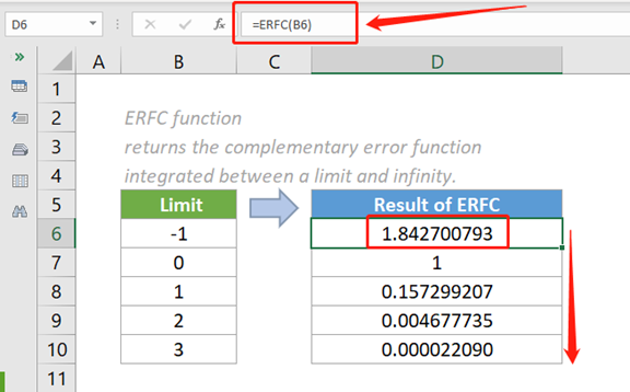
This article describes the formula syntax and usage of the ERFC function in Microsoft Excel.
Description
Returns the complementary ERF function integrated between x and infinity.
Syntax
ERFC(x)
The ERFC function syntax has the following arguments:
-
X Required. The lower bound for integrating ERFC.
Remarks
-
If x is nonnumeric, ERFC returns the #VALUE! error value.
Example
Copy the example data in the following table, and paste it in cell A1 of a new Excel worksheet. For formulas to show results, select them, press F2, and then press Enter. If you need to, you can adjust the column widths to see all the data.
|
Formula |
Description |
Result |
|
=ERFC(1) |
Complementary ERF function of 1. |
0.15729921 |
Need more help?
Содержание
- 1. Функция math.erf(x). Функция ошибок
- 2. Функция math.erfc(x). Дополнительная функция ошибок
- 3. Функция math.gamma(x). Гамма-функция
- 4. Функция math.lgamma(x). Натуральный логарифм от гамма-функции
- 5. Константа math.pi. Число π
- 6. Константа math.e. Экспонента
- 7. Константа math.tau. Число 2·π
- 8. Константа math.inf. Положительная бесконечность
- 9. Константа math.nan. Значение NaN (not a number)
- Связанные темы
Поиск на других ресурсах:
1. Функция math.erf(x). Функция ошибок
Функция math.erf(x) в языке Python предназначена для вычисления функции ошибок от аргумента x. Функция ошибок еще называется функцией ошибок Гаусса и определяется по формуле

Более подробно об особенностях использования функции ошибок можно узнать из других источников.
Пример.
# Функция math.erf(x)
import math

x = 1.5
y = math.erf(x) # y = 0.9661051464753108

x = 0
y = math.erf(x) # y = 0.0
⇑
2. Функция math.erfc(x). Дополнительная функция ошибок
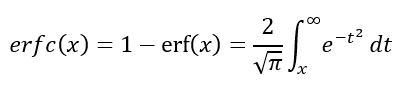
Функция math.erfc(x) используется для вычисления дополнительной функции ошибки в точке x. Дополнительная функция ошибки определяется как
1.0 - math.erf(x)
Функция math.erfc(x) используется в случаях, если значения x есть большими. При больших значениях x может произойти потеря значимости. Во избежание этого используется данная функция.
Функция math.erfc(x) используется в Python начиная с версии 3.2.
Пример.
# Функция math.erfc(x)
import math

x = 1.5
y = math.erfc(x) # y = 0.033894853524689274

x = 0
y = math.erfc(x) # y = 1.0
⇑
3. Функция math.gamma(x). Гамма функция
Функция math.gamma(x) возвращает Гамма-функцию от аргумента x. Гамма-функция вычисляется по формуле:

Более подробную информацию об использовании Гамма-функции можно найти в других источниках.
Функция math.gamma(x) введена в Python начиная с версии 3.2.
Пример.
# Функция math.gamma(x)
import math

x = 1.0
y = math.gamma(x) # y = 1.0

x = -2.2
y = math.gamma(x) # y = -2.2049805184191333

x = 3.8
y = math.gamma(x) # y = 4.694174205740421
⇑
4. Функция math.lgamma(x). Натуральный логарифм от гамма-функции
Функция math.lgamma(x) возвращает натуральный логарифм абсолютного значения Гамма-функции от аргумента x. Данная функция введена в Python начиная с версии 3.2.
Пример.
# Функция math.lgamma(x)
import math

x = 1.0
y = math.lgamma(x) # y = 0.0

x = 2.7
y = math.lgamma(x) # y = 0.4348205536551042
⇑
5. Константа math.pi. Число π
Константа math.pi определяет число π с доступной точностью.
Пример.
# Константа math.pi
import math

y = math.pi # y = 3.141592653589793

# Вычисление площади круга
r = 2.0
s = math.pi*r*r # s = 12.566370614359172
⇑
6. Константа math.e. Экспонента
Константа math.e определяет значение экспоненты с доступной точностью.
Пример.
# Константа math.e - экспонента
import math

y = math.e # y = 2.718281828459045

x = 1.5
y = math.e**x # y = 4.4816890703380645
⇑
7. Константа math.tau. Число 2·π
Константа math.tau определяет число 2·π с доступной точностью. Значение math.tau равно отношению длины окружности к ее радиусу. Константа используется в Python начиная с версии 3.6.
Пример.
# Константа math.tau
import math

y = math.tau # y = 6.283185307179586

# Вычисление длины окружности радиуса r = 2
r = 2.0
length = math.tau*r # length = 12.566370614359172
⇑
8. Константа math.inf. Положительная бесконечность
Константа math.inf определяет положительную бесконеченость с плавающей запятой. Чтобы определить отрицательную бесконечность, нужно использовать –math.inf.
Константа math.inf равна значению
float('inf')
Константа введена в Python начиная с версии 3.5.
Пример.
# Константа math.inf
import math
y = math.inf # y = inf - положительная бесконечность
print('y = ', y)

y = float('inf') # y = inf
print('y = ', y)
После запуска программы будет получен следующий результат
y = inf
y = inf
⇑
9. Константа math.nan. Значение NaN (not a number)
Константа math.nan введена в Python версии 3.6 и равна значению NaN с плавающей запятой. Значение NaN может возникать в случаях, когда результат вычисления неопределен. Примером такого вычисления может быть деление ноль на ноль, умножение ноль на бесконечность.
Определить, принимает ли результат значение NaN можно также с помощью функции math.isnan(x).
Константа math.nan введена в Python начиная с версии 3.5. Значение константы эквивалентно значению
float('nan')
Пример.
# Константа math.nan
import math

y = math.nan # y = nan
print('y = ', y)

y = float('nan') # y = nan
print('y = ', y)
Результат выполнения программы:
y = nan
y = nan
⇑
Связанные темы
- Теоретико-числовые функции и функции представления
- Степенные и логарифмические функции
- Тригонометрические функции
- Гиперболические функции
⇑
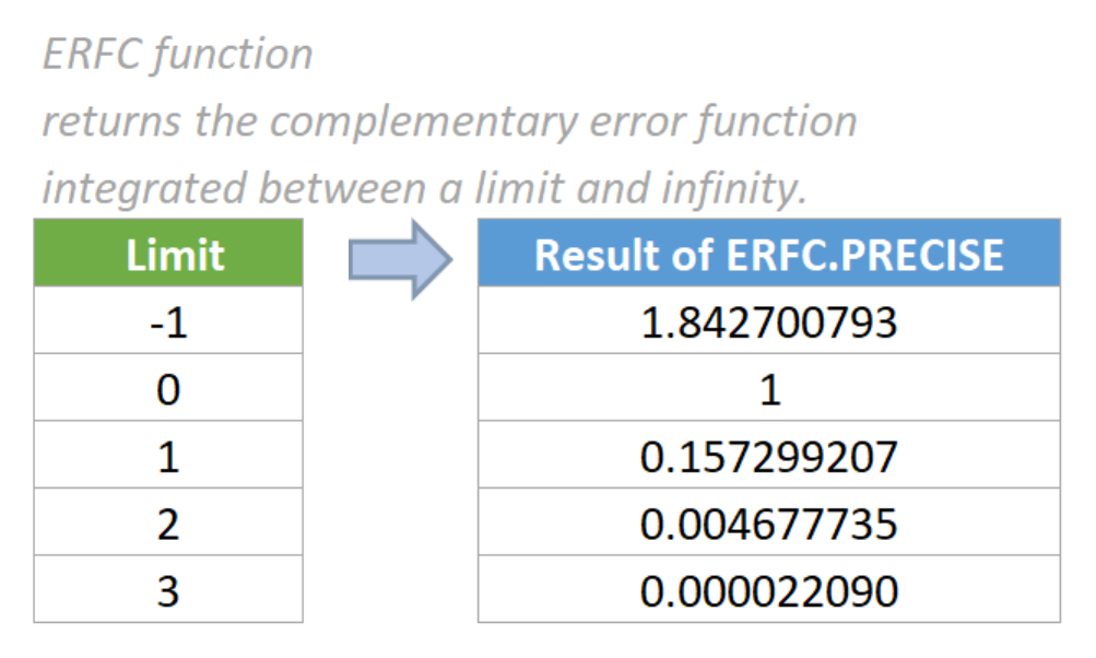
Функция ERFC возвращает дополнительную функцию ошибки, интегрированную между нижним пределом и бесконечностью.
Синтаксис
=ERFC (x)
аргументы
- X (обязательно): нижний предел интеграции ERFC.
Возвращаемое значение
Функция ERFC возвращает числовое значение.
Примечания к функциям
- Функция ERFC была улучшена в Excel 2010 и теперь может вычислять отрицательные значения.
В Excel 2007 функция ERFC принимает только положительные значения. Если предоставленный аргумент является отрицательным значением, функция ERFC вернет #ЧИСЛО! значение ошибки. - Значение! значение ошибки возникает, если предоставленный аргумент x не является числовым.
- Значение! значение ошибки возникает, если предоставленный аргумент x не является числовым.
- Функция ERFC всегда возвращает положительный результат в диапазоне от 0 до 2, независимо от того, является ли предоставленный аргумент положительным или отрицательным.
- Уравнение дополнительной функции ошибок:
Примеры
Чтобы вычислить дополнительную функцию ошибки, интегрированную между нижним пределом, указанным в таблице ниже, и бесконечным значением, выполните следующие действия.
1. Пожалуйста, скопируйте приведенную ниже формулу в ячейку D6, затем нажмите клавишу Enter, чтобы получить результат.
=ERFC (B6)
2. Выберите эту ячейку результатов и перетащите ее маркер автозаполнения вниз, чтобы получить остальные результаты.
Заметки:
- Когда единственный аргумент x равен нулю (0), ERFC возвращает в качестве результата 1.
- Аргумент в каждой из приведенных выше формул предоставляется в виде ссылки на ячейку, содержащей числовое значение.
- Мы также можем напрямую ввести значение в формулу. Например, формулу в ячейке D6 можно изменить на:
=ERFC (-1)
Относительные функции:
-
Excel EVEN Функция
Функция EVEN округляет числа от нуля до ближайшего четного целого числа.
-
Excel EXP Функция
Функция EXP возвращает результат возведения константы e в энную степень.
Лучшие инструменты для работы в офисе
Kutools for Excel — поможет вам выделиться из толпы
Хотите быстро и качественно выполнять свою повседневную работу? Kutools for Excel предлагает мощные расширенные функции 300 (объединение книг, суммирование по цвету, разделение содержимого ячеек, преобразование даты и т. д.) и экономит для вас 80% времени.
- Разработан для 1500 рабочих сценариев, помогает решить 80% проблем с Excel.
- Уменьшите количество нажатий на клавиатуру и мышь каждый день, избавьтесь от усталости глаз и рук.
- Станьте экспертом по Excel за 3 минуты. Больше не нужно запоминать какие-либо болезненные формулы и коды VBA.
- 30-дневная неограниченная бесплатная пробная версия. 60-дневная гарантия возврата денег. Бесплатное обновление и поддержка 2 года.
")
Вкладка Office — включение чтения и редактирования с вкладками в Microsoft Office (включая Excel)
- Одна секунда для переключения между десятками открытых документов!
- Уменьшите количество щелчков мышью на сотни каждый день, попрощайтесь с рукой мыши.
- Повышает вашу продуктивность на 50% при просмотре и редактировании нескольких документов.
- Добавляет эффективные вкладки в Office (включая Excel), точно так же, как Chrome, Firefox и новый Internet Explorer.
")
Комментарии (0)
Оценок пока нет. Оцените первым!
Оставляйте свои комментарии
График функции
В математике функция ошибок (также называемая Функция ошибок Гаусса ), часто обозначаемая erf, является сложной функцией комплексной определяемой как:
- erf z = 2 π ∫ 0 ze — t 2 dt. { displaystyle operatorname {erf} z = { frac {2} { sqrt { pi}}} int _ {0} ^ {z} e ^ {- t ^ {2}} , dt.}

Этот интеграл является особой (не элементарной ) и сигмоидной функцией, которая часто встречается в статистике вероятность, и уравнения в частных производных. Во многих из этих приложений аргумент функции является действительным числом. Если аргумент функции является действительным, значение также является действительным.
В статистике для неотрицательных значений x функция имеет интерпретацию: для случайной величины Y, которая нормально распределена с среднее 0 и дисперсия 1/2, erf x — это вероятность того, что Y попадает в диапазон [-x, x].
Две связанные функции: дополнительные функции ошибок (erfc ), определенная как
- erfc z = 1 — erf z, { displaystyle operatorname {erfc} z = 1- operatorname {erf} z,}
и функция мнимой ошибки (erfi ), определяемая как
- erfi z = — i erf (iz), { displaystyle operatorname {erfi} z = -i operatorname {erf} (iz),}

, где i — мнимая единица.
Содержание
- 1 Имя
- 2 Приложения
- 3 Свойства
- 3.1 Ряд Тейлора
- 3.2 Производная и интеграл
- 3.3 Ряд Бюрмана
- 3.4 Обратные функции
- 3.5 Асимптотическое разложение
- 3.6 Разложение на непрерывную дробь
- 3,7 Интеграл функции ошибок с функцией плотности Гаусса
- 3.8 Факториальный ряд
- 4 Численные приближения
- 4.1 Аппроксимация с элементарными функциями
- 4.2 Полином
- 4.3 Таблица значений
- 5 Связанные функции
- 5.1 функция дополнительных ошибок
- 5.2 Функция мнимой ошибки
- 5.3 Кумулятивная функци я распределения на
- 5.4 Обобщенные функции ошибок
- 5.5 Итерированные интегралы дополнительных функций ошибок
- 6 Реализации
- 6.1 Как действующая функция действительного аргумента
- 6.2 Как комплексная функция комплексного аргумента
- 7 См. Также
- 7.1 Связанные функции
- 7.2 Вероятность
- 8 Ссылки
- 9 Дополнительная литература
- 10 Внешние ссылки
Имя
Название «функция ошибки» и его аббревиатура erf были предложены Дж. В. Л. Глейшер в 1871 г. по причине его связи с «теорией вероятности, и особенно теорией ошибок ». Дополнение функции ошибок также обсуждалось Глейшером в отдельной публикации в том же году. Для «закона удобства» ошибок плотность задана как
- f (x) = (c π) 1 2 e — cx 2 { displaystyle f (x) = left ({ frac {c } { pi}} right) ^ { tfrac {1} {2}} e ^ {- cx ^ {2}}}

(нормальное распределение ), Глейшер вычисляет вероятность ошибки, лежащей между p { displaystyle p}

- (c π) 1 2 ∫ pqe — cx 2 dx = 1 2 (erf (qc) — erf (pc)). { displaystyle left ({ frac {c} { pi}} right) ^ { tfrac {1} {2}} int _ {p} ^ {q} e ^ {- cx ^ {2} } dx = { tfrac {1} {2}} left ( operatorname {erf} (q { sqrt {c}}) — operatorname {erf} (p { sqrt {c}}) right).}

Приложения
Когда результаты серии измерений описываются нормальным распределением со стандартным отклонением σ { displaystyle sigma}

Функции и дополнительные функции ошибок возникают, например, в решениях уравнения теплопроводности, когда граничные ошибки задаются ступенчатой функцией Хевисайда.
Функция ошибок и ее приближения Программу присвоили себе преподавателей, которые получили с высокой вероятностью или с низкой вероятностью. Дана случайная величина X ∼ Norm [μ, σ] { displaystyle X sim operatorname {Norm} [ mu, sigma]}![X sim operatorname {Norm} [ му, sigma]](https://wikimedia.org/api/rest_v1/media/math/render/svg/84024bc6827355ec6d23a062283a26d54b29698d)

- Pr [X ≤ L ] = 1 2 + 1 2 erf (L — μ 2 σ) ≈ A ехр (- B (L — μ σ) 2) { Displaystyle Pr [X Leq L] = { frac {1} {2 }} + { frac {1} {2}} operatorname {erf} left ({ frac {L- mu} {{ sqrt {2}} sigma}} right) приблизительно A exp left (-B left ({ frac {L- mu} { sigma}} right) ^ {2} right)}
![{ displaystyle Pr [X leq L ] = { frac {1} {2}} + { frac {1} {2}} operatorname {erf} left ({ frac {L- mu} {{ sqrt {2}} sigma }} right) приблизительно A exp left (-B left ({ frac {L- mu} { sigma}} right) ^ {2} right)}](https://wikimedia.org/api/rest_v1/media/math/render/svg/a72302c46832449e128a4d4e1adb28b514131270)
где A и B — верх числовые константы. Если L достаточно далеко от среднего, то есть μ — L ≥ σ ln k { displaystyle mu -L geq sigma { sqrt { ln {k}}}}
- Pr [X ≤ L] ≤ A exp (- B ln k) = A К B { displaystyle Pr [X leq L] leq A exp (-B ln {k}) = { frac {A} {k ^ {B}}}}
, поэтому становится вероятность 0 при k → ∞ { displaystyle k to infty}
Свойства
Графики на комплексной плоскости  Интегрируем exp (-z)
  erf (z)
Свойство erf (- z) = — erf (z) { displaystyle operatorname {erf} (-z) = — operatorname {erf} (z)}

Для любого комплексное число z:
- erf (z ¯) = erf (z) ¯ { displaystyle operatorname {erf} ({ overline {z}}) = { overline { operatorname {erf} (z)}}}

где z ¯ { displaystyle { overline {z}}}
Подынтегральное выражение f = exp (−z) и f = erf (z) показано в комплексной плоскости z на рисунках 2 и 3. Уровень Im (f) = 0 показан жирным зеленым цветом. линия. Отрицательные целые значения Im (f) показаны жирными красными линиями. Положительные целые значения Im (f) показаны толстыми синими линиями. Промежуточные уровни Im (f) = проявляются тонкими зелеными линиями. Промежуточные уровни Re (f) = показаны тонкими красными линиями для отрицательных значений и тонкими синими линиями для положительных значений.
Функция ошибок при + ∞ равна 1 (см. интеграл Гаусса ). На действительной оси erf (z) стремится к единице при z → + ∞ и к −1 при z → −∞. На мнимой оси он стремится к ± i∞.
Серия Тейлора
Функция ошибок — это целая функция ; у него нет сингулярностей (кроме бесконечности), и его разложение Тейлора всегда сходится, но, как известно, «[…] его плохая сходимость, если x>1».
определяющий интеграл нельзя вычислить в закрытой форме в терминах элементарных функций, но путем расширения подынтегрального выражения e в его ряд Маклорена и интегрирована почленно, можно получить ряд Маклорена функции ошибок как:
- erf (z) = 2 π ∑ n = 0 ∞ (- 1) nz 2 n + 1 n! (2 n + 1) знак равно 2 π (z — z 3 3 + z 5 10 — z 7 42 + z 9 216 — ⋯) { displaystyle operatorname {erf} (z) = { frac {2} { sqrt { pi}}} sum _ {n = 0} ^ { infty} { frac {(-1) ^ {n} z ^ {2n + 1}} {n! (2n + 1)}} = { frac {2} { sqrt { pi}}} left (z — { frac {z ^ {3}} {3}} + { frac {z ^ { 5}} {10}} — { frac {z ^ {7}} {42}} + { frac {z ^ {9}} {216}} — cdots right)}

, которое выполняется для каждого комплексного числа г. Члены знаменателя представляют собой последовательность A007680 в OEIS.
Для итеративного вычисления нового ряда может быть полезна следующая альтернативная формулировка:
- erf (z) = 2 π ∑ n = 0 ∞ (z ∏ К знак равно 1 N — (2 К — 1) Z 2 К (2 К + 1)) знак равно 2 π ∑ N = 0 ∞ Z 2 N + 1 ∏ К = 1 N — Z 2 К { Displaystyle OperatorName { erf} (z) = { frac {2} { sqrt { pi}}} sum _ {n = 0} ^ { infty} left (z prod _ {k = 1} ^ {n} { frac {- (2k-1) z ^ {2}} {k (2k + 1)}} right) = { frac {2} { sqrt { pi}}} sum _ {n = 0} ^ { infty} { frac {z} {2n + 1}} prod _ {k = 1} ^ {n} { frac {-z ^ {2}} {k}}}

потому что что — (2 k — 1) z 2 k (2 k + 1) { displaystyle { frac {- (2k-1) z ^ {2}} {k (2k + 1))}} }
Функция мнимой ошибки имеет очень похожий ряд Маклорена:
- erfi (z) = 2 π ∑ n = 0 ∞ z 2 n + 1 n! (2 n + 1) знак равно 2 π (z + z 3 3 + z 5 10 + z 7 42 + z 9 216 + ⋯) { displaystyle operatorname {erfi} (z) = { frac {2} { sqrt { pi}}} sum _ {n = 0} ^ { infty} { frac {z ^ {2n + 1}} {n! (2n + 1)}} = { frac {2} { sqrt { pi}}} left (z + { frac {z ^ {3}} {3}} + { frac {z ^ { 5}} {10}} + { frac {z ^ {7}} {42}} + { frac {z ^ {9}} {216}} + cdots right)}

, которое выполняется для любого комплексного числа z.
Производная и интеграл
Производная функция ошибок сразу следует из ее определения:
- ddz erf (z) = 2 π e — z 2. { displaystyle { frac {d} {dz}} operatorname {erf} (z) = { frac {2} { sqrt { pi}}} e ^ {- z ^ {2}}.}

Отсюда немедленно вычисляется производная функция мнимой ошибки :
- ddz erfi (z) = 2 π ez 2. { displaystyle { frac {d} {dz}} operatorname {erfi} (z) = { frac {2} { sqrt { pi }}} e ^ {z ^ {2}}.}

первообразная функции ошибок, которые можно получить посредством интегрирования по частям, составляет
- z erf (z) + е — z 2 π. { displaystyle z operatorname {erf} (z) + { frac {e ^ {- z ^ {2}}} { sqrt { pi}}}.}

Первообразная мнимой функции ошибок, также можно получить интегрированием по частям:
- z erfi (z) — ez 2 π. { displaystyle z operatorname {erfi} (z) — { frac {e ^ {z ^ {2}}} { sqrt { pi}}}.}

Производные высшего порядка задаются как
- erf (k) (z) = 2 (- 1) k — 1 π H k — 1 (z) e — z 2 = 2 π dk — 1 dzk — 1 (e — z 2), k = 1, 2, … { Displaystyle operatorname {erf} ^ {(k)} (z) = { frac {2 (-1) ^ {k-1}} { sqrt { pi}}} { mathit {H} } _ {k-1} (z) e ^ {- z ^ {2}} = { frac {2} { sqrt { pi}}} { frac {d ^ {k-1}} {dz ^ {k-1}}} left (e ^ {- z ^ {2}} right), qquad k = 1,2, dots}

где H { displaystyle { mathit {H}}}
ряд Бюрмана
Расширение, которое сходится быстрее для всех реальных значений x { displaystyle x}
- erf (x) = 2 π sgn (x) 1 — e — x 2 (1 — 1 12 ( 1 — e — x 2) — 7 480 (1 — e — x 2) 2 — 5 896 (1 — e — x 2) 3 — 787 276480 (1 — e — x 2)) 4 — ⋯) знак равно 2 π знак (x) 1 — e — x 2 (π 2 + ∑ k = 1 ∞ cke — kx 2). { displaystyle { begin {align} operatorname {erf} (x) = { frac {2} { sqrt { pi}}} operatorname {sgn} (x) { sqrt {1-e ^ {-x ^ {2}}}} left (1 — { frac {1} {12}} left (1-e ^ {- x ^ {2}} right) — { frac {7} {480}} left (1-e ^ {- x ^ {2}} right) ^ {2} — { frac {5} {896}} left (1-e ^ {- x ^ {2 }} right) ^ {3} — { frac {787} {276480}} left (1-e ^ {- x ^ {2}} right) ^ {4} — cdots right) \ [10pt] = { frac {2} { sqrt { pi}}} operatorname {sgn} (x) { sqrt {1-e ^ {- x ^ {2}}}} left ({ frac { sqrt { pi}} {2}} + sum _ {k = 1} ^ { infty} c_ {k} e ^ {- kx ^ {2}} right). end {выровнено}}
![{ displaystyle { begin {align} operatorname {erf} (x) = { frac {2} { sqrt { pi}}} operatorname {sgn} (x) { sqrt {1-e ^ {- x ^ {2}}}} left (1 - { frac {1} {12}} left (1 -e ^ {- x ^ {2}} right) - { frac {7} {480}} left (1-e ^ {- x ^ {2}} right) ^ {2} - { frac {5} {896}} left (1-e ^ {- x ^ {2}} right) ^ {3} - { frac {787} {276480}} left (1-e ^ {- x ^ {2 }} right) ^ {4} - cdots right) \ [10pt] = { frac {2} { sqrt { pi}}} operatorname {sgn} (x) { sqrt {1 -e ^ {- x ^ {2}}}} left ({ frac { sqrt { pi}} {2}} + sum _ {k = 1} ^ { infty} c_ {k} e ^ {- kx ^ {2}} right). end {align}}}](https://wikimedia.org/api/rest_v1/media/math/render/svg/24ddba05e595a553fee25644a3542188281bd844)
Сохраняя только первые два коэффициента и выбирая c 1 = 31 200 { displaystyle c_ {1} = { frac {31} {200}}}


- erf (x) ≈ 2 π sign (x) 1 — e — x 2 (π 2 + 31 200 e — x 2 — 341 8000 e — 2 х 2). { displaystyle operatorname {erf} (x) приблизительно { frac {2} { sqrt { pi}}} operatorname {sgn} (x) { sqrt {1-e ^ {- x ^ {2 }}}} left ({ frac { sqrt { pi}} {2}} + { frac {31} {200}} e ^ {- x ^ {2}} — { frac {341} {8000}} e ^ {- 2x ^ {2}} right).}

Обратные функции
Обратная функция
Учитывая комплексное число z, не существует уникального комплексного числа w, удовлетворяющего erf (w) = z { displaystyle operatorname {erf} (w) = z}

- erf (erf — 1 ( х)) = х. { displaystyle operatorname {erf} left ( operatorname {erf} ^ {- 1} (x) right) = x.}

Обратная функция ошибок обычно определяется с помощью домена (- 1,1), и он ограничен этой областью многих систем компьютерной алгебры. Однако его можно продолжить и на диск | z | < 1 of the complex plane, using the Maclaurin series
- erf — 1 (z) знак равно ∑ К знак равно 0 ∞ ck 2 k + 1 (π 2 z) 2 k + 1, { displaystyle operatorname {erf} ^ {- 1} (z) = sum _ {k = 0} ^ { infty} { frac {c_ {k}} {2k + 1}} left ({ frac { sqrt { pi}} {2}} z right) ^ {2k + 1},}

где c 0 = 1 и
- ck = ∑ m = 0 k — 1 cmck — 1 — m (m + 1) (2 m + 1) = {1, 1, 7 6, 127 90, 4369 2520, 34807 16200,…}. { displaystyle c_ {k} = sum _ {m = 0} ^ {k-1} { frac {c_ {m} c_ {k-1-m}} {(m + 1) (2m + 1) }} = left {1,1, { frac {7} {6}}, { frac {127} {90}}, { frac {4369} {2520}}, { frac {34807} {16200}}, ldots right }.}

Итак, у нас есть разложение в ряд (общие множители были удалены из числителей и знаменателей):
- erf — 1 (z) = 1 2 π ( z + π 12 z 3 + 7 π 2 480 z 5 + 127 π 3 40320 z 7 + 4369 π 4 5806080 z 9 + 34807 π 5 182476800 z 11 + ⋯). { displaystyle operatorname {erf} ^ {- 1} (z) = { tfrac {1} {2}} { sqrt { pi}} left (z + { frac { pi} {12} } z ^ {3} + { frac {7 pi ^ {2}} {480}} z ^ {5} + { frac {127 pi ^ {3}} {40320}} z ^ {7} + { frac {4369 pi ^ {4}} {5806080}} z ^ {9} + { frac {34807 pi ^ {5}} {182476800}} z ^ {11} + cdots right). }

(После отмены дроби числителя / знаменателя характерми OEIS : A092676 / OEIS : A092677 в OEIS ; без отмены членов числителя в записи OEIS : A002067.) Значение функции ошибок при ± ∞ равно ± 1.
Для | z | < 1, we have erf (erf — 1 (z)) = z { displaystyle operatorname {erf} left ( operatorname {erf} ^ {- 1} (z) right) = z}
обратная дополнительная функция ошибок определяется как
- erfc — 1 (1 — z) = erf — 1 (z). { displaystyle operatorname {erfc} ^ {- 1} (1-z) = operatorname {erf} ^ {- 1} (z).}

Для действительного x существует уникальное действительное число erfi — 1 (x) { displaystyle operatorname {erfi} ^ {- 1} (x)}

Для любого действительного x, Метод Ньютона можно использовать для вычислений erfi — 1 (x) { displaystyle operatorname {erfi} ^ {- 1} (x)}
- erfi — 1 (z) = ∑ k = 0 ∞ (- 1) ККК 2 К + 1 (π 2 Z) 2 К + 1, { Displaystyle OperatorName {erfi} ^ {- 1} (г) = сумма _ {к = 0} ^ { infty} { гидроразрыва {(-1) ^ {k} c_ {k}} {2k + 1}} left ({ frac { sqrt { pi}} {2}} z right) ^ {2k + 1},}

, где c k определено, как указано выше.
Асимптотическое разложение
Полезным асимптотическим разложением дополнительные функции (и, следовательно, также и функции ошибок) для больших вещественных x
- erfc (x) = e — x 2 x π [1 + ∑ n = 1 ∞ (- 1) n 1 ⋅ 3 ⋅ 5 ⋯ (2 n — 1) (2 x 2) n] = e — x 2 x π ∑ n = 0 ∞ (- 1) п (2 п — 1)! ! (2 х 2) n, { displaystyle operatorname {erfc} (x) = { frac {e ^ {- x ^ {2}}} {x { sqrt { pi}}}} left [1 + sum _ {n = 1} ^ { infty} (- 1) ^ {n} { frac {1 cdot 3 cdot 5 cdots (2n-1)} {(2x ^ {2}) ^ {n}}} right] = { frac {e ^ {- x ^ {2}}} {x { sqrt { pi}}}} sum _ {n = 0} ^ { infty} ( -1) ^ {n} { frac {(2n-1) !!} {(2x ^ {2}) ^ {n}}},}
![{ displaystyle operatorname {erfc} (x) = { frac {e ^ {- x ^ {2}}} {x { sqrt { pi}}}} left [1+ sum _ {n = 1} ^ { infty} (-1) ^ {n} { frac {1 cdot 3 cdot 5 cdots (2n-1)} {(2x ^ {2}) ^ { n}}} right] = { frac {e ^ {-x ^ {2}}} {x { sqrt { pi}}}} sum _ {n = 0} ^ { infty} (- 1) ^ {n} { frac {(2n-1) !!} {(2x ^ {2}) ^ {n}}},}](https://wikimedia.org/api/rest_v1/media/math/render/svg/7fc8c3aefff3ba787b080c5186dd3aec8ec76ef9)
где (2n — 1) !! — это двойной факториал числа (2n — 1), которое является произведением всех нечетных чисел до (2n — 1). Этот ряд расходуется для любого конечного x, и его значение как асимптотического разложения состоит в том, что для любого N ∈ N { displaystyle N in mathbb {N}}
- erfc (Икс) знак равно е — Икс 2 Икс π ∑ N знак равно 0 N — 1 (- 1) N (2 N — 1)! ! (2 х 2) n + RN (x) { displaystyle operatorname {erfc} (x) = { frac {e ^ {- x ^ {2}}} {x { sqrt { pi}}}} sum _ {n = 0} ^ {N-1} (- 1) ^ {n} { frac {(2n-1) !!} {(2x ^ {2}) ^ {n}}} + R_ {N} (x)}

где остаток в нотации Ландау равен
- RN (x) = O (x 1 — 2 N e — x 2) { displaystyle R_ {N} ( x) = O left (x ^ {1-2N} e ^ {- x ^ {2}} right)}

при x → ∞. { displaystyle x to infty.}

Действительно, точное значение остатка равно
- R N (x): = (- 1) N π 2 1 — 2 N (2 N)! N! ∫ Икс ∞ T — 2 N e — T 2 dt, { Displaystyle R_ {N} (x): = { frac {(-1) ^ {N}} { sqrt { pi}}} 2 ^ { 1-2N} { frac {(2N)!} {N!}} Int _ {x} ^ { infty} t ^ {- 2N} e ^ {- t ^ {2}} , dt,}

который легко следует по индукции, записывая
- e — t 2 = — (2 t) — 1 (e — t 2) ′ { displaystyle e ^ {- t ^ {2}} = — (2t) ^ {- 1} left (e ^ {- t ^ {2}} right) ‘}
и интегрирование по частям.
Для достаточно больших значений x, только первые несколько этих асимптотических разностей необходимы, чтобы получить хорошее приближение erfc (x) (в то время как для не слишком больших значений x приведенное выше разложение Тейлора при 0 обеспечивает очень быструю сходимость).
Расширение непрерывной дроби
A Разложение непрерывной дроби дополнительные функции ошибок:
- erfc (z) = z π e — z 2 1 z 2 + a 1 1 + a 2 z 2 + a 3 1 + ⋯ am = м 2. { displaystyle operatorname {erfc} (z) = { frac {z} { sqrt { pi}}} e ^ {- z ^ {2}} { cfrac {1} {z ^ {2} + { cfrac {a_ {1}} {1 + { cfrac {a_ {2}} {z ^ {2} + { cfrac {a_ {3}} {1+) dotsb}}}}}}}} qquad a_ {m} = { frac {m} {2}}.}

Интеграл функции ошибок с функцией плотности Гаусса
- ∫ — ∞ ∞ erf (ax + б) 1 2 π σ 2 е — (Икс — μ) 2 2 σ 2 dx знак равно erf [a μ + b 1 + 2 a 2 σ 2], a, b, μ, σ ∈ R { displaystyle int _ {- infty} ^ { infty} operatorname {erf} left (ax + b right) { frac {1} { sqrt {2 pi sigma ^ {2}}}} e ^ {- { frac {(x- mu) ^ {2}} {2 sigma ^ {2}}}} , dx = operatorname {erf} left [{ frac {a mu + b } { sqrt {1 + 2a ^ {2} sigma ^ {2}}} right], qquad a, b, mu, sigma in mathbb {R}}
![{ displaystyle int _ {- infty} ^ { infty} operatorname {erf} left (ax + b right) { frac {1} { sqrt {2 pi sigma ^ {2}}}} e ^ {- { frac {(x- mu) ^ {2}} {2 sigma ^ {2}}}} , dx = operatorname {erf} left [{ frac {a mu + b} { sqrt {1 + 2a ^ {2} sigma ^ {2}}} right], qquad a, b, му, sigma in mathbb {R}}](https://wikimedia.org/api/rest_v1/media/math/render/svg/9b6adc2c661b24b44dc1e3d7e16be70023daacd8)
Факториальный ряд
- Обратное:
-
- erfc z = e — z 2 π z ∑ n = 0 ∞ (- 1) n Q n (z 2 + 1) n ¯ = e — z 2 π z (1 — 1 2 1 (z 2 + 1) + 1 4 1 (z 2 + 1) (z 2 + 2) — ⋯) { displaystyle { begin {align} operatorname {erfc} z = { frac {e ^ {- z ^ {2}}} {{ sqrt { pi}} , z}} sum _ {n = 0} ^ { infty} { frac {(-1) ^ {n} Q_ {n}} {{(z ^ {2} + 1)} ^ { ba r {n}}}} \ = { frac {e ^ {- z ^ {2}}} {{ sqrt { pi}} , z}} left ( 1 — { frac {1} {2}} { frac {1} {(z ^ {2} +1)}} + { frac {1} {4}} { frac {1} {(z ^ {2} +1) (z ^ {2} +2)}} — cdots right) end {align}}}
- erfc z = e — z 2 π z ∑ n = 0 ∞ (- 1) n Q n (z 2 + 1) n ¯ = e — z 2 π z (1 — 1 2 1 (z 2 + 1) + 1 4 1 (z 2 + 1) (z 2 + 2) — ⋯) { displaystyle { begin {align} operatorname {erfc} z = { frac {e ^ {- z ^ {2}}} {{ sqrt { pi}} , z}} sum _ {n = 0} ^ { infty} { frac {(-1) ^ {n} Q_ {n}} {{(z ^ {2} + 1)} ^ { ba r {n}}}} \ = { frac {e ^ {- z ^ {2}}} {{ sqrt { pi}} , z}} left ( 1 — { frac {1} {2}} { frac {1} {(z ^ {2} +1)}} + { frac {1} {4}} { frac {1} {(z ^ {2} +1) (z ^ {2} +2)}} — cdots right) end {align}}}
- сходится для Re (z 2)>0. { displaystyle operatorname {Re} (z ^ {2})>0.}
Здесь
- Q n = def 1 Γ (1/2) ∫ 0 ∞ τ (τ — 1) ⋯ ( τ — n + 1) τ — 1/2 е — τ d τ знак равно ∑ К знак равно 0 N (1 2) к ¯ s (n, k), { displaystyle Q_ {n} { stackrel { text {def}} {=}} { frac {1} { Gamma (1/2)}} int _ {0} ^ { infty} tau ( tau -1) cdots ( tau -n + 1) tau ^ {-1/2} e ^ {- tau} d tau = sum _ {k = 0} ^ {n} left ({ frac {1} {2}} right) ^ { bar {k}} s (n, k),}
- Q n = def 1 Γ (1/2) ∫ 0 ∞ τ (τ — 1) ⋯ ( τ — n + 1) τ — 1/2 е — τ d τ знак равно ∑ К знак равно 0 N (1 2) к ¯ s (n, k), { displaystyle Q_ {n} { stackrel { text {def}} {=}} { frac {1} { Gamma (1/2)}} int _ {0} ^ { infty} tau ( tau -1) cdots ( tau -n + 1) tau ^ {-1/2} e ^ {- tau} d tau = sum _ {k = 0} ^ {n} left ({ frac {1} {2}} right) ^ { bar {k}} s (n, k),}
- zn ¯ { displaystyle z ^ { bar {n}}}
обозначает возрастающий факториал, а s (n, k) { displaystyle s (n, k)}
обозначает знаковое число Стирлинга первого рода.

- Представление бесконечной суммой, составляющей двойной факториал :
-
- ERF (Z) знак равно 2 π ∑ N знак равно 0 ∞ (- 2) N (2 N — 1)! (2 N + 1)! Z 2 N + 1 { Displaystyle OperatorName {ERF} (г) = { frac {2} { sqrt { pi}}} sum _ {n = 0} ^ { infty} { frac {( -2) ^ {n} (2n-1) !!} {(2n + 1)!}} Z ^ {2n + 1}}
- ERF (Z) знак равно 2 π ∑ N знак равно 0 ∞ (- 2) N (2 N — 1)! (2 N + 1)! Z 2 N + 1 { Displaystyle OperatorName {ERF} (г) = { frac {2} { sqrt { pi}}} sum _ {n = 0} ^ { infty} { frac {( -2) ^ {n} (2n-1) !!} {(2n + 1)!}} Z ^ {2n + 1}}

Численные приближения
Приближение элементов сарными функциями
- Абрамовиц и Стегун дают несколько приближений с точностью (уравнения 7.1.25–28). Это позволяет выбрать наиболее быстрое приближение, подходящее для данного приложения. В порядке увеличения точности они следующие:
-
- erf (x) ≈ 1 — 1 (1 + a 1 x + a 2 x 2 + a 3 x 3 + a 4 x 4) 4, x ≥ 0 { displaystyle имя оператора {erf} (x) приблизительно 1 — { frac {1} {(1 + a_ {1} x + a_ {2} x ^ {2} + a_ {3} x ^ {3} + a_ { 4} x ^ {4}) ^ {4}}}, qquad x geq 0}
- erf (x) ≈ 1 — 1 (1 + a 1 x + a 2 x 2 + a 3 x 3 + a 4 x 4) 4, x ≥ 0 { displaystyle имя оператора {erf} (x) приблизительно 1 — { frac {1} {(1 + a_ {1} x + a_ {2} x ^ {2} + a_ {3} x ^ {3} + a_ { 4} x ^ {4}) ^ {4}}}, qquad x geq 0}
- (максимальная ошибка: 5 × 10)

- , где a 1 = 0,278393, a 2 = 0,230389, a 3 = 0,000972, a 4 = 0,078108
-
- erf (x) ≈ 1 — (a 1 t + a 2 t 2 + a 3 t 3) e — x 2, t = 1 1 + px, x ≥ 0 { displaystyle operatorname {erf} (x) приблизительно 1- (a_ {1} t + a_ {2} t ^ {2} + a_ {3} t ^ {3}) e ^ {- x ^ {2}}, quad t = { frac {1} {1 + px}}, qquad x geq 0}
(максимальная ошибка: 2,5 × 10)
- erf (x) ≈ 1 — (a 1 t + a 2 t 2 + a 3 t 3) e — x 2, t = 1 1 + px, x ≥ 0 { displaystyle operatorname {erf} (x) приблизительно 1- (a_ {1} t + a_ {2} t ^ {2} + a_ {3} t ^ {3}) e ^ {- x ^ {2}}, quad t = { frac {1} {1 + px}}, qquad x geq 0}
- где p = 0,47047, a 1 = 0,3480242, a 2 = -0,0958798, a 3 = 0,7478556
-
- erf (x) ≈ 1 — 1 (1 + a 1 x + a 2 x 2 + ⋯ + a 6 x 6) 16, x ≥ 0 { displaystyle operatorname {erf} (x) приблизительно 1 — { frac {1} {(1 + a_ {1} x + a _ {2} x ^ {2} + cdots + a_ {6} x ^ {6}) ^ {16}}}, qquad x geq 0}
(максимальная ошибка: 3 × 10)
- erf (x) ≈ 1 — 1 (1 + a 1 x + a 2 x 2 + ⋯ + a 6 x 6) 16, x ≥ 0 { displaystyle operatorname {erf} (x) приблизительно 1 — { frac {1} {(1 + a_ {1} x + a _ {2} x ^ {2} + cdots + a_ {6} x ^ {6}) ^ {16}}}, qquad x geq 0}
- , где a 1 = 0,0705230784, a 2 = 0,0422820123, a 3 = 0,0092705272, a 4 = 0,0001520143, a 5 = 0,0002765672, a 6 = 0,0000430638
-
- erf (x) ≈ 1 — (a 1 t + a 2 t 2 + ⋯ + a 5 t 5) e — x 2, t = 1 1 + px { displaystyle operatorname {erf} (x) приблизительно 1- (a_ {1} t + a_ {2} t ^ {2} + cdots + a_ {5} t ^ {5}) e ^ {- x ^ {2}}, quad t = { frac {1} {1 + px}}}
(максимальная ошибка: 1,5 × 10)
- erf (x) ≈ 1 — (a 1 t + a 2 t 2 + ⋯ + a 5 t 5) e — x 2, t = 1 1 + px { displaystyle operatorname {erf} (x) приблизительно 1- (a_ {1} t + a_ {2} t ^ {2} + cdots + a_ {5} t ^ {5}) e ^ {- x ^ {2}}, quad t = { frac {1} {1 + px}}}
- , где p = 0,3275911, a 1 = 0,254829592, a 2 = −0,284496736, a 3 = 1,421413741, a 4 = −1,453152027, a 5 = 1,061405429
- Все эти приближения действительны для x ≥ 0 Чтобы использовать эти приближения для отрицательного x, викорируйте тот факт, что erf (x) — нечетная функция, поэтому erf (x) = −erf (−x).
- Экспоненциальные границы и чисто экспоненциальное приближение для дополнительных функций задаются как
-
- erfc (x) ≤ 1 2 e — 2 x 2 + 1 2 e — x 2 ≤ e — x 2, x>0 erfc ( х) ≈ 1 6 е — х 2 + 1 2 е — 4 3 х 2, х>0. { displaystyle { begin {align} operatorname {erfc} (x) leq { frac {1} {2}} e ^ {- 2x ^ {2}} + { frac {1} {2} } e ^ {- x ^ {2}} leq e ^ {- x ^ {2}}, qquad x>0 \ имя оператора {erfc} (x) приблизительно { frac {1} { 6}} e ^ {- x ^ {2}} + { frac {1} {2}} e ^ {- { frac {4} {3}} x ^ {2}}, qquad x>0. end {align}}}
- erfc (x) ≤ 1 2 e — 2 x 2 + 1 2 e — x 2 ≤ e — x 2, x>0 erfc ( х) ≈ 1 6 е — х 2 + 1 2 е — 4 3 х 2, х>0. { displaystyle { begin {align} operatorname {erfc} (x) leq { frac {1} {2}} e ^ {- 2x ^ {2}} + { frac {1} {2} } e ^ {- x ^ {2}} leq e ^ {- x ^ {2}}, qquad x>0 \ имя оператора {erfc} (x) приблизительно { frac {1} { 6}} e ^ {- x ^ {2}} + { frac {1} {2}} e ^ {- { frac {4} {3}} x ^ {2}}, qquad x>0. end {align}}}

-
- erfc (x) ≈ (1 — e — A x) e — x 2 B π х. { displaystyle operatorname {erfc} left (x right) приблизительно { frac { left (1-e ^ {- Ax} right) e ^ {- x ^ {2}}} {B { sqrt { pi}} x}}.}
- erfc (x) ≈ (1 — e — A x) e — x 2 B π х. { displaystyle operatorname {erfc} left (x right) приблизительно { frac { left (1-e ^ {- Ax} right) e ^ {- x ^ {2}}} {B { sqrt { pi}} x}}.}

- Они определили {A, B} = {1.98, 1.135}, { displaystyle {A, B } = {1.98,1.135 },}
, что дает хорошее приближение для всех x ≥ 0. { displaystyle x geq 0.}

- Одноканальная нижняя граница:
-
- erfc (x) ≥ 2 e π β — 1 β е — β Икс 2, Икс ≥ 0, β>1, { Displaystyle OperatorName {erfc} (x) geq { sqrt { frac {2e} { pi}}} { frac { sqrt { beta -1}} { beta}} e ^ {- beta x ^ {2}}, qquad x geq 0, beta>1,}
- erfc (x) ≥ 2 e π β — 1 β е — β Икс 2, Икс ≥ 0, β>1, { Displaystyle OperatorName {erfc} (x) geq { sqrt { frac {2e} { pi}}} { frac { sqrt { beta -1}} { beta}} e ^ {- beta x ^ {2}}, qquad x geq 0, beta>1,}

- где параметр β может быть выбран, чтобы минимизировать ошибку на желаемом интервале приближения.
- Другое приближение дано Сергеем Виницким с использованием его «глобальных приближений Паде»:
-
- erf (x) ≈ sgn (x) 1 — exp (- x 2 4 π + ax 2 1 + ax 2) { displaystyle operatorname {erf} (x) приблизительно Operatorname {sgn} (x) { sqrt {1- exp left (-x ^ {2} { frac {{ frac {4} { pi) })} + ax ^ {2}} {1 + ax ^ {2}}} right)}}}
- erf (x) ≈ sgn (x) 1 — exp (- x 2 4 π + ax 2 1 + ax 2) { displaystyle operatorname {erf} (x) приблизительно Operatorname {sgn} (x) { sqrt {1- exp left (-x ^ {2} { frac {{ frac {4} { pi) })} + ax ^ {2}} {1 + ax ^ {2}}} right)}}}

- где
-
- a = 8 (π — 3) 3 π (4 — π) ≈ 0, 140012. { displaystyle a = { frac {8 ( pi -3)} {3 pi (4- pi)}} приблизительно 0,140012.}
- a = 8 (π — 3) 3 π (4 — π) ≈ 0, 140012. { displaystyle a = { frac {8 ( pi -3)} {3 pi (4- pi)}} приблизительно 0,140012.}
- Это сделано так, чтобы быть очень точным в окрестностях 0 и добавление бесконечности, а относительная погрешность меньше 0,00035 для всех действительных x. Использование альтернативного значения ≈ 0,147 снижает максимальную относительную ошибку примерно до 0,00013.
- Это приближение можно инвертировать, чтобы получить приближение для других функций ошибок:
-
- erf — 1 (x) ≈ sgn (x) (2 π a + ln (1 — x 2) 2) 2 — ln (1 — x 2) a — (2 π a + ln (1 — x 2) 2). { displaystyle operatorname {erf} ^ {- 1} (x) приблизительно operatorname {sgn} (x) { sqrt {{ sqrt { left ({ frac {2} { pi a}} + { frac { ln (1-x ^ {2})} {2}} right) ^ {2} — { frac { ln (1-x ^ {2})} {a}}}} — left ({ frac {2} { pi a}} + { frac { ln (1-x ^ {2})} {2}} right)}}.}
- erf — 1 (x) ≈ sgn (x) (2 π a + ln (1 — x 2) 2) 2 — ln (1 — x 2) a — (2 π a + ln (1 — x 2) 2). { displaystyle operatorname {erf} ^ {- 1} (x) приблизительно operatorname {sgn} (x) { sqrt {{ sqrt { left ({ frac {2} { pi a}} + { frac { ln (1-x ^ {2})} {2}} right) ^ {2} — { frac { ln (1-x ^ {2})} {a}}}} — left ({ frac {2} { pi a}} + { frac { ln (1-x ^ {2})} {2}} right)}}.}

Многочлен
Приближение с максимальной ошибкой 1,2 × 10⁻⁷ { displaystyle 1,2 times 10 ^ {- 7}}
- erf ( x) = {1 — τ x ≥ 0 τ — 1 x < 0 {displaystyle operatorname {erf} (x)={begin{cases}1-tau xgeq 0\tau -1x<0end{cases}}}

с
- τ = t ⋅ exp (- x 2 — 1,26551223 + 1,00002368 t + 0,37409196 t 2 + 0,09678418 t 3 — 0,18628806 t 4 + 0,27886807 t 5 — 1,13520398 t 6 + 1,48851587 t 7 — 0,82215223 t 8 + 0,17087277 t 9) { displaystyle { begin {align} tau = t cdot exp left (-x ^ {2} -1,26551223 + 1,00002368 t + 0,37409196t ^ {2} + 0,09678418t ^ {3} -0,18628806t ^ {4} вправо. \ left. qquad qquad qquad + 0,27886807t ^ {5} -1,13520398t ^ {6} + 1,48851587t ^ {7} -0,82215223t ^ {8} + 0,17087 277t ^ {9} right) end {align}}}
и
- t = 1 1 + 0,5 | х |. { displaystyle t = { frac {1} {1 + 0,5 | x |}}.}

Таблица значений
| x | erf(x) | 1-erf (x) |
|---|---|---|
| 0 | 0 | 1 |
| 0,02 | 0,022564575 | 0,977435425 |
| 0,04 | 0,045111106 | 0,954888894 |
| 0,06 | 0,067621594 | 0, 932378406 |
| 0,08 | 0.090078126 | 0,909921874 |
| 0,1 | 0,112462916 | 0,887537084 |
| 0,2 | 0,222702589 | 0,777297411 |
| 0,3 | 0,328626759 | 0,671373241 |
| 0, 4 | 0,428392355 | 0,571607645 |
| 0,5 | 0,520499878 | 0,479500122 |
| 0,6 | 0.603856091 | 0,396143909 |
| 0,7 | 0,677801194 | 0,322198806 |
| 0,8 257> | 0,742100965 | 0,257899035 |
| 0,9 | 0,796908212 | 0,203091788 |
| 1 | 0,842700793 | 0, 157299207 |
| 1,1 | 0,88020507 | 0,11979493 |
| 1,2 | 0,910313978 | 0,089686022 |
| 1,3 | 0,934007945 | 0,065992055 |
| 1,4 | 0.95228512 | 0,04771488 |
| 1,5 | 0, 966105146 | 0,033894854 |
| 1,6 | 0,976348383 | 0,023651617 |
| 1,7 | 0,983790459 | 0,016209541 |
| 1,8 | 0,989090502 | 0,010909498 |
| 1,9 | 0,992790429 | 0,007209571 |
| 2 | 0,995322265<25767> | 0,00477 |
| 2.1 | 0.997020533 | 0.002979467 |
| 2.2 | 0.998137154 | 0,001862846 |
| 2,3 | 0,998856823 | 0,001143177 |
| 2,4 | 0,999311486 | 0,000688514 |
| 2,5 | 0.999593048 | 0.000406952 |
| 3 | 0.99997791 | 0,00002209 |
| 3,5 | 0,999999257 | 0,000000743 |
Связанные функции
Дополнительная функция
дополнительная функция ошибок, обозначается erfc { displaystyle mathrm {erfc}}
- erfc (x) = 1 — erf (x) = 2 π ∫ x ∞ e — t 2 dt знак равно е — Икс 2 erfcx (х), { displaystyle { begin {выровнено} OperatorName {erfc} (x) = 1- operatorname {erf} (x) \ [5p t] = { frac {2} { sqrt { pi}}} int _ {x} ^ { infty} e ^ {- t ^ {2}} , dt \ [5pt] = e ^ {- x ^ {2}} operatorname {erfcx} (x), end {align}}}
![{ displaystyle { begin {align} operatorname {erfc} (x) = 1- operatorname {erf} (x) \ [5pt ] = { frac {2} { sqrt { pi}}} int _ {x} ^ { infty} e ^ {- t ^ {2}} , dt \ [5pt] = e ^ {- x ^ {2}} operatorname {erfcx} (x), end {align}}}](https://wikimedia.org/api/rest_v1/media/math/render/svg/8808e6f3ad9aab23f14d55db707a39388d256788)
, который также определяет erfcx { displaystyle mathrm {erfcx} }

- erfc (x ∣ x ≥ 0) = 2 π ∫ 0 π / 2 exp (- x 2 sin 2 θ) d θ. { displaystyle operatorname {erfc} (x mid x geq 0) = { frac {2} { pi}} int _ {0} ^ { pi / 2} exp left (- { frac {x ^ {2}} { sin ^ {2} theta}} right) , d theta.}

Это выражение действительно только для положительных значений x, но его можно использовать вместе с erfc (x) = 2 — erfc (−x), чтобы получить erfc (x) для отрицательных значений. Эта форма выгодна тем, что диапазон интегрирования является фиксированным и конечным. Расширение этого выражения для erfc { displaystyle mathrm {erfc}}
- erfc (x + y ∣ x, y ≥ 0) = 2 π ∫ 0 π / 2 ехр (- x 2 sin 2 θ — y 2 cos 2 θ) d θ. { displaystyle operatorname {erfc} (x + y mid x, y geq 0) = { frac {2} { pi}} int _ {0} ^ { pi / 2} exp left (- { frac {x ^ {2}} { sin ^ {2} theta}} — { frac {y ^ {2}} { cos ^ {2} theta}} right) , d theta.}

Функция мнимой ошибки
мнимой ошибки, обозначаемая erfi, обозначает ошибки как
- erfi (x) = — i erf (ix) Знак равно 2 π ∫ 0 xet 2 dt знак равно 2 π ex 2 D (x), { displaystyle { begin {align} operatorname {erfi} (x) = — i operatorname {erf} (ix) \ [ 5pt] = { frac {2} { sqrt { pi}}} int _ {0} ^ {x} e ^ {t ^ {2}} , dt \ [5pt] = { frac {2} { sqrt { pi}}} e ^ {x ^ {2}} D (x), end {align}}}
![{ displaystyle { begin {align} operatorname {erfi} (x) = - i operatorname {erf} (ix) \ [5pt] = { frac {2} { sqrt { pi}}} int _ {0} ^ {x} e ^ {t ^ {2 }} , dt \ [5pt] = { frac {2} { sqrt { pi}}} e ^ {x ^ {2}} D (x), end {align}}}](https://wikimedia.org/api/rest_v1/media/math/render/svg/4480a8ec17e274a7ad6b8ef25cc76234d48c0433)
где D (x) — функция Доусона (который можно использовать вместо erfi, чтобы избежать арифметического переполнения ).
Несмотря на название «функция мнимой ошибки», erfi (x) { displaystyle operatorname {erfi} (x)}
Функция Когда ошибки оценивается для произвольных сложных аргументов z, результирующая комплексная функция ошибок обычно обсуждается в масштабированной форме как функция Фаддеева :
- w (z) = e — z 2 erfc (- iz) = erfcx (- iz). { displaystyle w (z) = e ^ {- z ^ {2}} operatorname {erfc} (-iz) = operatorname {erfcx} (-iz).}
Кумулятивная функция распределения
Функция ошибок по существующей стандартной стандартной функции нормального кумулятивного распределения, обозначаемой нормой (x) в некоторых языках программного обеспечения, поскольку они отличаются только масштабированием и переводом. Действительно,
- Φ (x) = 1 2 π ∫ — ∞ xe — t 2 2 dt = 1 2 [1 + erf (x 2)] = 1 2 erfc (- x 2) { displaystyle Phi (x) = { frac {1} { sqrt {2 pi}}} int _ {- infty} ^ {x} e ^ { tfrac {-t ^ {2}} {2}} , dt = { frac {1} {2}} left [1+ operatorname {erf} left ({ frac {x} { sqrt {2}}} right) right] = { frac {1} {2}} operatorname {erfc} left (- { frac {x} { sqrt {2}}} right)}
![{ displaystyle Phi (x) = { frac {1} { sqrt {2 pi}}} int _ {- infty} ^ {x } e ^ { tfrac {-t ^ {2}} {2}} , dt = { frac {1} {2}} left [1+ operatorname {erf} left ({ frac {x } { sqrt {2}}} right) right] = { frac {1} {2}} operatorname {erfc} left (- { frac {x} { sqrt {2}}} справа)}](https://wikimedia.org/api/rest_v1/media/math/render/svg/e19dc7206f8b3b571e81153816c478abd91a679e)
или переставлен для erf и erfc:
- erf ( x) = 2 Φ (x 2) — 1 erfc (x) = 2 Φ (- x 2) = 2 (1 — Φ (x 2)). { displaystyle { begin {align} operatorname {erf} (x) = 2 Phi left (x { sqrt {2}} right) -1 \ operatorname {erfc} (x) = 2 Phi left (-x { sqrt {2}} right) = 2 left (1- Phi left (x { sqrt {2}} right) right). End {выравнивается} }}

Следовательно, функция ошибок также тесно связана с Q-функцией, которая является вероятностью хвоста стандартного нормального распределения. Q-функция может быть выражена через функцию ошибок как
- Q (x) = 1 2 — 1 2 erf (x 2) = 1 2 erfc (x 2). { displaystyle Q (x) = { frac {1} {2}} — { frac {1} {2}} operatorname {erf} left ({ frac {x} { sqrt {2}}) } right) = { frac {1} {2}} operatorname {erfc} left ({ frac {x} { sqrt {2}}} right).}

Обратное значение из Φ { displaystyle Phi}
- пробит (p) = Φ — 1 (p) = 2 erf — 1 (2 p — 1) = — 2 erfc — 1 (2 p). { displaystyle operatorname {probit} (p) = Phi ^ {- 1} (p) = { sqrt {2}} operatorname {erf} ^ {- 1} (2p-1) = — { sqrt {2}} operatorname {erfc} ^ {- 1} (2p).}
Стандартный нормальный cdf чаще используется в вероятности и статистике, а функция ошибок чаще используется в других разделах математики.
Функция ошибки является частным случаем функции Миттаг-Леффлера и может также быть выражена как сливающаяся гипергеометрическая функция (функция Куммера):
- erf (х) знак равно 2 х π M (1 2, 3 2, — х 2). { displaystyle operatorname {erf} (x) = { frac {2x} { sqrt { pi}}} M left ({ frac {1} {2}}, { frac {3} {2 }}, — x ^ {2} right).}

Он имеет простое выражение в терминах интеграла Френеля.
В терминах регуляризованной гамма-функции P и неполная гамма-функция,
- erf (x) = sgn (x) P (1 2, x 2) = sgn (x) π γ (1 2, x 2). { displaystyle operatorname {erf} (x) = operatorname {sgn} (x) P left ({ frac {1} {2}}, x ^ {2} right) = { frac { operatorname {sgn} (x)} { sqrt { pi}}} gamma left ({ frac {1} {2}}, x ^ {2} right).}

sgn (x) { displaystyle operatorname {sgn} (x)}
Обобщенные функции ошибок
График обобщенных функций ошибок E n (x):. серая кривая: E 1 (x) = (1 — e) /
π { displaystyle scriptstyle { sqrt { pi}}}

Некоторые авторы обсуждают более общие функции:
- E n (x) = n! π ∫ 0 Икс е — Т N д т знак равно N! π ∑ п знак равно 0 ∞ (- 1) п Икс N п + 1 (N п + 1) п!. { displaystyle E_ {n} (x) = { frac {n!} { sqrt { pi}}} int _ {0} ^ {x} e ^ {- t ^ {n}} , dt = { frac {n!} { sqrt { pi}}} sum _ {p = 0} ^ { infty} (- 1) ^ {p} { frac {x ^ {np + 1}} {(np + 1) p!}}.}

Примечательные случаи:
- E0(x) — прямая линия, проходящая через начало координат: E 0 (x) = xe π { displaystyle textstyle E_ {0} (x) = { dfrac {x} {e { sqrt { pi}}}}}
- E2(x) — функция, erf (x) ошибки.

После деления на n!, все E n для нечетных n выглядят похожими (но не идентичными) друг на друга. Аналогично, E n для четного n выглядят похожими (но не идентичными) друг другу после простого деления на n!. Все обобщенные функции ошибок для n>0 выглядят одинаково на положительной стороне x графика.
Эти обобщенные функции могут быть эквивалентно выражены для x>0 с помощью гамма-функции и неполной гамма-функции :
- E n (x) = 1 π Γ (n) (Γ (1 n) — Γ (1 n, xn)), x>0. { displaystyle E_ {n} (x) = { frac {1} { sqrt { pi}}} Gamma (n) left ( Gamma left ({ frac {1} {n}} right) — Gamma left ({ frac {1} {n}}, x ^ {n} right) right), quad quad x>0.}

Следовательно, мы можем определить ошибку функция в терминах неполной гамма-функции:
- erf (x) = 1 — 1 π Γ (1 2, x 2). { displaystyle operatorname {erf} (x) = 1 — { frac {1} { sqrt { pi}}} Gamma left ({ frac {1} {2}}, x ^ {2} right).}

Итерированные интегралы дополнительных функций
Повторные интегралы дополнительные функции ошибок определения как
- inerfc (z) = ∫ z ∞ in — 1 erfc (ζ) d ζ i 0 erfc (z) = erfc (z) i 1 erfc (z) = ierfc (z) знак равно 1 π е — z 2 — z erfc (z) я 2 erfc (z) = 1 4 [erfc (z) — 2 z ierfc (z)] { displaystyle { begin {align } operatorname {i ^ {n} erfc} (z) = int _ {z} ^ { infty} operatorname {i ^ {n-1} erfc} ( zeta) , d zeta \ имя оператора {i ^ {0} erfc} (z) = operatorname {erfc} (z) \ operatorname {i ^ {1} erfc} (z) = operat orname {ierfc} (z) = { frac { 1} { sqrt { pi}}} e ^ {- z ^ {2}} — z operatorname {erfc} (z) \ operatorname {i ^ {2} erfc} (z) = { frac {1} {4}} left [ operatorname {erfc} (z) -2z operatorname {ierfc} (z) right] \ end {выровнено}}
![{ displaystyle { begin {align} operatorname { i ^ {n} erfc} (z) = int _ {z} ^ { infty} operatorname {i ^ {n-1} erfc} ( zeta) , d zeta \ имя оператора {i ^ {0} erfc} (z) = operatorname {erfc} (z) \ operatorname {i ^ {1} erfc} (z) = operatorname {ierfc} (z) = { frac {1} { sqrt { pi}}} e ^ {- z ^ {2}} - z operatorname {erfc} (z) \ operatorname {i ^ {2} erfc} (z) = { frac { 1} {4}} left [ operatorname {erfc} (z) -2z operatorname {ierfc} (z) right] \ конец {выровнено}}}](https://wikimedia.org/api/rest_v1/media/math/render/svg/66b57abb0a01139b31a14f5a8d651e4aa2e5f4f2)
Общая рекуррентная формула:
- 2 ninerfc (z) = in — 2 erfc (z) — 2 цинк — 1 erfc (z) { displaystyle 2n operatorname {i ^ {n} erfc} (z) = operatorname {i ^ { n-2} erfc} (z) -2z operatorname {i ^ {n-1} erfc} (z)}

У них есть степенной ряд
- в erfc (z) = ∑ j = 0 ∞ (- Z) J 2 N — JJ! Γ (1 + N — J 2), { displaystyle i ^ {n} operatorname {erfc} (z) = sum _ {j = 0} ^ { infty} { frac {(-z) ^ { j}} {2 ^ {nj} j! Gamma left (1 + { frac {nj} {2}} right)}},}

из следуют свойства симметрии
- i 2 m ERFC (- Z) знак равно — я 2 m ERFC (Z) + ∑ Q знак равно 0 мZ 2 д 2 2 (м — д) — 1 (2 д)! (м — д)! { displaystyle i ^ {2m} operatorname {erfc} (-z) = — i ^ {2m} operatorname {erfc} (z) + sum _ {q = 0} ^ {m} { frac {z ^ {2q}} {2 ^ {2 (mq) -1} (2q)! (Mq)!}}}

и
- i 2 m + 1 erfc (- z) = i 2 m + 1 erfc (г) + ∑ ä знак равно 0 ìZ 2 ä + 1 2 2 ( м — д) — 1 (2 д + 1)! (м — д)!. { displaystyle i ^ {2m + 1} operatorname {erfc} (-z) = i ^ {2m + 1} operatorname {erfc} (z) + sum _ {q = 0} ^ {m} { гидроразрыва {z ^ {2q + 1}} {2 ^ {2 (mq) -1} (2q + 1)! (mq)!}}.}

Реализации
Как действительная функция вещественного аргумента
- В операционных системах, совместимых с Posix, заголовок math.h должен являть, а математическая библиотека libm должна быть функция erf и erfc (двойная точность ), а также их одинарная точность и расширенная точность аналоги erff, erfl и erfc, erfcl.
- Библиотека GNU Scientific предоставляет функции erf, erfc, log (erf) и масштабируемые функции ошибок.
Как сложная функция комплексного аргумента
- libcerf, числовая библиотека C для сложных функций, предоставляет комплексные функции cerf, cerfc, cerfcx и реальные функции erfi, erfcx с точностью 13–14 цифр на основе функции Фаддеева, реализованной в пакете MIT Faddeeva Package
См. также
Связанные ции
- интеграл Гаусса, по всей действительной прямой
- функция Гаусса, производная
- функция Доусона, перенормированная функция мнимой ошибки
- интеграл Гудвина — Стона
по вероятности
- Нормальное распределение
- Нормальная кумулятивная функция распределения, масштабированная и сдвинутая форма функций ошибок
- Пробит, обратная или квантильная функция нормального CDF
- Q-функция, вероятность хвоста нормального распределения
Ссылки
Дополнительная литература
- Abramowitz, Milton ; Стегун, Ирен Энн, ред. (1983) [июнь 1964]. «Глава 7». Справочник по математическим функциям с формулами, графики и математическими таблицами. Прикладная математика. 55 (Девятое переиздание с дополнительными исправлениями; десятое оригинальное издание с исправлениями (декабрь 1972 г.); первое изд.). Вашингтон.; Нью-Йорк: Министерство торговли США, Национальное бюро стандартов; Dover Publications. п. 297. ISBN 978-0-486-61272-0 . LCCN 64-60036. MR 0167642. LCCN 65-12253.
- Press, William H.; Теукольский, Саул А.; Веттерлинг, Уильям Т.; Фланнери, Брайан П. (2007), «Раздел 6.2. Неполная гамма-функция и функция ошибок », Числовые рецепты: Искусство научных вычислений (3-е изд.), Нью-Йорк: Cambridge University Press, ISBN 978-0-521- 88068-8
- Темме, Нико М. (2010), «Функции ошибок, интегралы Доусона и Френеля», в Олвер, Фрэнк У. Дж. ; Лозье, Даниэль М.; Бойсверт, Рональд Ф.; Кларк, Чарльз В. (ред.), Справочник NIST по математическим функциям, Cambridge University Press, ISBN 978-0-521-19225-5 , MR 2723248
Внешние ссылки
- MathWorld — Erf
- Таблица интегралов функций ошибок
Время чтения 3 мин.
Метод Python math.erf() вернет ошибку в точке x. Функция ошибки также известна как функция ошибки Гаусса: она выдает ошибку, если в качестве параметра передается любое не числовое значение.
Python math.erfc() — это встроенный метод, определенный в математическом модуле, который используется для поиска дополнительной функции ошибок в точке x, если x — переданный параметр. Например, если x передается в качестве параметра в функцию erf(erf(x)), она возвращает дополнительную функцию ошибки.
Содержание
- Что такое функция erf() в Python?
- Синтаксис
- Параметры
- Возвращаемое значение
- Примеры программ по методу erf() в Python
- Пример 1. Программа, демонстрирующая работу метода erf()
- Пример 2. Программа для передачи значения вне допустимого диапазона из функции и отображения вывода
- Что такое функция erfc() в Python?
- Синтаксис
- Параметры
- Возвращаемое значение
- Примеры программ
- Пример 1. Программа, показывающая работу метода erfc()
- Пример 2. Передача значения вне допустимого диапазона из функции и отображения вывода
Python erf() — это встроенный метод, определенный в математическом модуле, который используется для поиска функции ошибки в точке x, если x является переданным параметром. Например, если x передается в качестве параметра в функцию erf(erf(x)), она возвращает функцию ошибки. Мы можем использовать математический модуль, импортировав его.
Синтаксис
Здесь var — это переменная, функцию ошибки которой мы должны найти.
Параметры
Имеет один аргумент var, который принимает значения числового типа данных и выдает TypeError, если передается аргумент любого другого типа данных.
Возвращаемое значение
Возвращает значение функции ошибки числа в типе данных float.
См. следующий пример кода.
|
import math var = 0.6 print(math.erf(var)) |
Примеры программ по методу erf() в Python
 | Math.erf() в примере Python")
Пример 1. Программа, демонстрирующая работу метода erf()
|
import math a1 = 0.3 b1 = 0.9 c1 = 0.7 d1 = 0.2 print(«Value for parameter «, a1, » is «, math.erf(a1)) print(«Value for parameter «, b1, » is «, math.erf(b1)) print(«Value for parameter «, c1, » is «, math.erf(c1)) print(«Value for parameter «, d1, » is «, math.erf(d1)) |
Выход:
|
Value for parameter 0.3 is 0.3286267594591274 Value for parameter 0.9 is 0.796908212422832 Value for parameter 0.7 is 0.6778011938374183 Value for parameter 0.2 is 0.22270258921047847 |
В этом примере кода мы видели, что, передавая параметр vaild, который отличается для разных примеров, мы получаем желаемое решение метода erf().
Пример 2. Программа для передачи значения вне допустимого диапазона из функции и отображения вывода
См. следующий код.
|
import math x = ‘b’ print(math.erf(x)) |
Выход:
|
TypeError: must be real number, not str |
В этом примере мы видим, что при передаче параметра, который не имеет числового типа, функция выдает ошибку.
Python erfc() — это встроенный метод, определенный в математическом модуле, который используется для поиска дополнительной функции ошибок в точке x, если x — переданный параметр. Например, если x передается в качестве параметра в функцию erf(erf(x)), она возвращает дополнительную функцию ошибки.
Что такое функция erfc() в Python?
Функция Python math.erfc() возвращает дополнительную функцию ошибки в точке x. Функция ошибки также известна как функция ошибки Гаусса, и функция выдает ошибку, если в качестве параметра передается любое не числовое значение. Определяется как 1,0 – erf(x). Используется для большого значения x, если мы вычтем из 1, то это приведет к потере значимости.
Мы можем использовать математический модуль, импортировав его. После импорта мы используем для вызова этой функции статический объект.
Синтаксис
Здесь var — это переменная, для которой мы должны найти дополнительную функцию ошибки.
Параметры
Он принимает один параметр var, который принимает значения числового типа данных и выдает ошибку типа, если передается аргумент любого другого типа данных.
Возвращаемое значение
Он возвращает значение функции ошибки числа в типе данных float.
См. следующий код.
|
import math var = 0.6 print(math.erfc(var)) |
Примеры программ
 | Math.erfc() в примере Python")
Пример 1. Программа, показывающая работу метода erfc()
|
import math a1 = 0.3 b1 = 0.9 c1 = 0.7 d1 = 0.2 print(«Value for parameter «, a1, » is «, math.erfc(a1)) print(«Value for parameter «, b1, » is «, math.erfc(b1)) print(«Value for parameter «, c1, » is «, math.erfc(c1)) print(«Value for parameter «, d1, » is «, math.erfc(d1)) |
Выход:
|
Value for parameter 0.3 is 0.6713732405408726 Value for parameter 0.9 is 0.20309178757716786 Value for parameter 0.7 is 0.32219880616258156 Value for parameter 0.2 is 0.7772974107895215 |
В этом примере мы видели, что, передавая параметр vaild, который отличается для разных примеров, мы получаем желаемое решение метода erfc(), которое является дополнительным значением функции ошибок.
Пример 2. Передача значения вне допустимого диапазона из функции и отображения вывода
|
import math x = ‘b’ print(math.erfc(x)) |
Выход:
|
TypeError: must be real number, not str |
В этом примере мы видели, что при передаче параметра, который не имеет числового типа, функция выдает ошибку.