Fec прямое исправление ошибок - Ремонт и установка крупной бытовой техники

Поскольку требования к полосе пропускания увеличиваются, а допуск на ошибки и задержку уменьшаются, разработчики систем передачи данных искали новые способы расширения доступной полосы пропускания и повышения качества передачи. Одно из решений на самом деле не ново, но оказалось весьма полезным. Это называется прямым исправлением ошибок (FEC), в течение многих лет этот метод использовался для обеспечения эффективной высококачественной передачи данных по шумным каналам. Сегодня с увеличением пропускной способности передачи данных и увеличением расстояния, давайте узнаем больше о методике FEC в оптических сетях.

Что такое FEC?

Прямая коррекция ошибок (FEC) — это метод цифровой обработки сигналов, используемый для повышения надежности данных. Это делается путем введения избыточных данных, называемых кодом с исправлением ошибок, перед передачей или хранением данных. FEC предоставляет приемнику возможность исправления ошибок без обратного канала для запроса повторной передачи данных. Как мы знаем, иногда оптические сигналы могут ухудшаться из-за некоторых факторов во время передачи, что может привести к неправильной оценке на стороне приемника, возможно, принятию сигнала «1» за сигнал «0» или сигнала «0» за сигнал «1». Если количество ошибок при передаче находится в пределах корректирующей способности (прерывистые ошибки), канальный декодер обнаружит и исправит ложные “0” или “1” для улучшения качества сигнала.

Рисунок 1. Принцип работы FEC

Развитие прямого исправления ошибок в оптической связи можно разделить на три поколения. FEC первого поколения представляет собой первое, которое будет успешно использоваться в подводных системах и наземных системах. По мере развития систем WDM в коммерческих системах был установлен более мощный FEC второго поколения. Появление FEC третьего поколения открыло новые перспективы для следующего поколения систем оптической связи.

Каковы типы и особенности FEC?

Типы

В настоящее время практические технологии FEC для SDH (синхронная цифровая иерархия) и DWDM (плотное мультиплексирование с разделением по длине волны) в основном следующие:

In-band FEC. In-band FEC поддерживается стандартом ITU-T G.707. Контролируемые символы кода FEC загружаются с использованием части служебных байтов в кадре SDH. Усиление кодирования невелико (3-4 дБ).Внеполосный FEC. Внеполосный FEC поддерживается стандартом ITU-T G.975/709.

Out-of-band FEC обладает большой избыточностью кодирования, возможностью исправления ошибок, высокой гибкостью и высоким коэффициентом усиления кодирования (5-6 дБ).

Enhanced FEC (EFEC). Enhanced FEC в основном используется в системах оптической связи, где требования к задержке не являются строгими, а требования по усилению кодирования особенно высоки. Хотя процесс кодирования и декодирования EFEC является более сложным и менее применимым в настоящее время, благодаря его преимуществам в производительности, он превратится в практическую технологию и станет основным направлением следующего поколения out-of-band FEC.

Характеристики

FEC уменьшает количество ошибок передачи, расширяет рабочий диапазон и снижает требования к питанию для систем связи. FEC также увеличивает эффективную пропускную способность системы, даже с дополнительными контрольными битами, добавленными к битам данных, устраняя необходимость повторной передачи данных, искаженных случайным шумом.

FEC самостоятельно повышает достоверность данных на приемнике. В рамках системного контекста FEC становится технологией, которую разработчик системы может использовать несколькими способами. Наиболее очевидным преимуществом использования FEC является использование систем с ограниченной мощностью. Однако посредством использования сигнализации более высокого порядка ограничения полосы пропускания также могут быть устранены. Во многих беспроводных системах допустимая мощность передатчика ограничена. Эти ограничения могут быть вызваны соблюдением стандарта или практическими соображениями. FEC позволяет передавать с гораздо более высокими скоростями передачи данных, если доступна дополнительная полоса пропускания.

Применение FEC в 100G сетях

В контексте оптоволоконных сетей FEC используется для определения оптического SNR (OSNR) — одного из ключевых параметров, определяющих, как далеко может пройти длина волны, прежде чем она нуждается в регенерации. FEC особенно важен при скоростях высокоскоростной передачи данных, где требуются усовершенствованные схемы модуляции, чтобы минимизировать дисперсию и соответствие сигнала с частотной сеткой. Без включения FEC транспорт 100G был бы ограничен чрезвычайно короткими расстояниями. Для реализации передачи на большие расстояния (> 2500 км) усиление системы должно быть дополнительно улучшено примерно на 2 дБ. Переход FEC с жесткого решения на мягкое решение восполняет этот пробел в производительности.

Поскольку стремление к все более высоким скоростям передачи продолжается, схемы прямого исправления ошибок (SD-FEC) становятся все более популярными. Хотя для этого может потребоваться около 20% байтов — почти в три раза больше, чем в исходной схеме кодирования RS — выгоды, которые они получают в контексте высокоскоростных сетей, значительны. Например, FEC, который приводит к усилению от 1 до 2 дБ в сети 100G, означает увеличение охвата на 20-40%.

Замечания для FEC в сетях 100G

Что следует учитывать при настройке FEC в 100G сетях? Предлагается обратить внимание на следующие советы.

Метод реализации

Некоторые специальные модули имеют свои собственные функции FEC, такие как FS 100G CFP конвертеры интерфейсов. В то время как 100G QSFP28 оптический модуль в основном полагается на конфигурацию функции FEC на устройстве для реализации исправления ошибок, таких как 100G коммутаторы.

Поддерживает ли коммутатор FEC

Конфигурирование FEC на 100G коммутаторах может быть достигнуто только в том случае, если коммутатор поддерживает его, и не все коммутаторы поддерживают это. В то время как все 100G коммутаторы поддерживают FEC, предоставляемые FS.

Тип коммутатора	Тип порта	Поддержка FEC или нет
S5850-48S2Q4C	4810Gb, 240Gb, 4*100Gb	Да (для оба 40Gb и 100Gb порты)
S8050-20Q4C	2040Gb, 4100Gb	Да (для оба 40Gb и 100Gb порты)
N8500-48B6C	4025Gb, 6100Gb	Да (для оба 25Gb и 100Gb порты)
N8500-32C	32*100Gb	Да

Таблица 1. Технические характеристики FS 100G коммутаторов

Внимание: для FS 100G коммутаторов функция FEC включена по умолчанию. Если требуется включить его после выключения, можно настроить команду FEC.

Включить ли FEC на QSFP28 100G модулях

Функция FEC — это не просто преимущество, процесс исправления кода ошибки неизбежно приведет к некоторой задержке пакета данных. Поэтому не все QSFP28 100G модули нуждаются в этом. Согласно стандартному протоколу IEEE не рекомендуется включать FEC при использовании QSFP28-LR4-100G модулей, за исключением того, что рекомендуется включать его. Поскольку технология QSFP28 100G модулей варьируется от компании к компании, поэтому ситуация не совсем одинакова. В следующей таблице объясняется, рекомендуется ли включать FEC при использовании FS 100G QSFP28 модулей.

Тип модуля	Описание	с FEC
QSFP28-SR4-100G	850nm 100m MTP/MPO Модуль для SMF	Нет
QSFP28-LR4-100G	1310nm 10km Модуль для SMF	Нет
QSFP28-PIR4-100G	1310nm 500m Модуль для SMF	Нет
QSFP28-IR4-100G	1310nm 2km Модуль для SMF	Да
QSFP28-EIR4-100G	1310nm 10km Модуль для SMF	Да
QSFP28-ER4-100G	1310nm 40km Модуль для SMF	Да

Таблица 2. Технические характеристики FS 100G QSFP28 модулей

Согласованность функций FEC на обоих концах канала

Функция FEC порта является частью автосогласования. Когда автоматическое согласование порта включено, функция FEC определяется согласованием на обоих концах канала. Если функция FEC включена на одном конце, другой конец должен также включить ее, в противном случае порт не работает.

Стекирование & FEC

Настройка команды FEC не поддерживается, если порт уже настроен как физически стековый порт.Наоборот, порты, которые были настроены с помощью команд FEC, не поддерживают настройку в качестве физического стекового члена.

Заключение

FEC стал критически важной в волоконно-оптической связи, так как магистральные сети увеличиваются в скорости до 40 и 100G, особенно в условиях плохой связи оптического сигнала с шумом. Такие среды становятся более распространенными в высокоскоростных средах, поскольку в сетях используется больше оптических усилителей. Со всеми этими событиями, FEC будет продолжать играть роль в будущих сетях. Для обеспечения нормальной работы сети рекомендуется обратить особое внимание на функцию FEC на оптических модулях, которая поможет вам повысить производительность при передаче данных.

Источник

High-capacity long-haul optical fiber transmission

Xiang Liu, in Optical Communications in the 5G Era, 2022

8.4.4 Capacity-approaching FEC

Forward-error correction is an important technology to enable a communication link to approach the Shannon limit. The use of FEC in optical fiber communication links has gone through three generations [94]

•: The first generation of FEC codes appeared in the 1987–93 period, and the representative FEC code is Reed–Solomon (RS) code (255,239) with a FEC overhead of 6.7% and a net coding gain (NCG) of 5.8 dB at an output BER of 10⁻¹⁵.
•: The second generation of FEC codes in the 2000–04 period, and the representative FEC codes are the concatenated codes, showing an NCG of 9.4 dB at an FEC overhead of ~25%.
•: The third generation of FEC codes started to be adopted in real systems around 2006, and the representative FEC codes are SD decoding enabled low-density parity check (LDPC) codes, turbo codes, etc., showing an NCG of over 10 dB at an FEC overhead of between ~15% and ~25%. The key feature of the third generation of FEC codes is the use of SD decoding [94].

A key performance indicator of FEC is its NCG, which is defined as

(8.27)NCGdB=10log10SNRBERout−10log10SNRBERin+10log10(R)

where BER_in is the maximally allowed input BER to the FEC to achieve a reference output BER of BER_out, SNR(x) is the SNR needed for a given modulation format to reach a BER of x without coding, and R is the FEC code rate. For BPSK modulation format, we have

(8.28)SNRBPSKBER=erfc−1(2BER)

where erfc⁻¹() is the inverse complementary error function. For QPSK modulation format, we have

(8.29)SNRQPSKBER=2erfc−1(2BER)

For 16-QAM modulation format, we have

(8.30)SNR16QAMBER=10erfc−1(83BER)

For high-speed transmission based on 16-QAM, multiple high-performance FEC codes have been studied. Table 8.1 shows some of the FEC codes and their performances. The first code is the concentrated FEC (CFEC) code adopted by the Optical Internetworking Forum (OIF) for 400ZR [95,96]. Its required BER_in for a BER_out of 10⁻¹⁵ is 1.22×10⁻², and its code rate is 0.871, leading to an NCG of 11.76 dB. The second code is an enhanced version of CFEC, named as CFEC+, which offers an increased NCG of 11.45 dB [97]. The third code is referred to as open FEC (OFEC), which was adopted by the Open ROADM Multisource Agreement (MSA) and was proposed to the ITU project on 200 G/400 G FlexO-LR for 450 km black link applications [98]. The OFEC offers a further increased NCG of 11.6 dB.

Table 8.1. High-performance FEC codes used for 16-QAM based high-speed transmission.

FEC code	BER_in (SNR_in) for BER_out=10⁻¹⁵*	Code rate	NCG
CFEC [95,96]	1.22×10⁻² (13.6 dB)	0.871	10.76 dB
CFEC+ [97]	1.81×10⁻² (12.9 dB)	0.871	11.45 dB
OFEC [98]	1.98×10⁻² (12.7 dB)	0.867	11.60 dB
A 20%-OH LDPC [57]	~2.76×10⁻² (12.0 dB)	0.833	12.12 dB
A 25%-OH LDPC [99]	~3.45×10⁻² (11.5 dB)	~0.8	~12.5 dB

FEC, forward-error correction; BER, bit error ratio; SNR, signal-to-noise ratio; NCG, net coding gain; LDPC, low-density parity check.

*: At the reference BER_out of 10⁻¹⁵, the corresponding SNR for 16-QAM is ~24.95 dB.

In a recent 800-Gb/second-per-wavelength demonstration, a 20% overhead (OH) LDPC code was used, and a high NCG of 12.12 dB was achieved [57]. Finally, a 25%-OH FEC was demonstrated in real-time 200-Gb/second coherent transceivers, achieving a remarkably high NCG of 12.5 dB [99]. Similar performance has also been shown in the 800-Gb/second demonstration when the LDPC FEC OH was increased to 25% [57].

It is worthwhile to compare the above FEC performances with the theoretical limit. The ultimate NCG can be derived from the Shannon’s capacity theorem. The channel capacity C of a binary symmetric channel with HD decoding is given as

(8.31)CHD=1+BERin·log2BERin+1−BERin·log21−BERin

where BER_in is the input BER threshold and the channel capacity C_HD can be set to the FEC code rate R [94]. For a given FEC code rate R, we can calculate BER_in. Together with Eqs. (8.27–8.30), we can then calculate the NCG for a given modulation format at a given reference BER_out.

For SD decoding, the capacity of a binary symmetric channel, which has two possible inputs X=A and X=−A, can be expressed as [35]

(8.32)CSD=12∫−∞+∞p(y|A)log2p(y|A)p(y)dy+12∫−∞+∞p(y|−A)log2p(y|−A)p(y)dy

where p(y|A) is the conditional probability of getting y at the receiver when the input is A, and p(y) is the probability of receiving y. Similar to the case with HD, for a given FEC code rate R=C_SD, we can calculate BER_in, from which we can then calculate the NCG for a given modulation format at a given reference BER_out. In the idealized case of SD decoding with infinite quantization bits, the NCG obtained by SD decoding is π/2 times as large as (or ~2 dB higher than) that obtained by HD decoding when R approaches zero.

Fig. 8.13 shows the Shannon limits of HD and SD NCGs for BPSK/QPSK, together with some recently demonstrated high-performance FEC codes. For HD decoding, KP4 and staircase FEC [100] are widely used in the optical communication industry. Remarkably, the staircase FEC offers a NCG of 9.41 dB, which is only 0.56 dB away from the HD Shannon limit [100]. For SD decoding, NCGs of 11.6 and 12.25 dB have been achieved with 20% and 33% OHs, respectively [57]. These SD NCGs are only about 1 dB away from the SD Shannon limit.

Figure 8.13. The Shannon limits of HD and SD NCGs for BPSK/QPSK and some recently demonstrated FEC codes [57,96,100]. The reference output BER (BER_out) is set at 10⁻¹⁵.

Fig. 8.14 shows the Shannon limits of HD and SD NCGs for 16-QAM, together with some recently demonstrated high-performance FEC codes. The Shannon limits of NCGs for 16-QAM are slightly higher than those for BPSK/QPSK. This can be understood by the slightly flatter BER curve of 16-QAM at high BER values as compared to BPSK/QPSK, as shown in Figure 7.6. For HD decoding, the staircase FEC is again only ~0.6 dB away from the HD Shannon limit. For SD decoding, the CFEC+, OFEC, 20%-OH LDPC, and 25%-OH LDPC described in Table 8.1 are all within 1.4 dB away from the SD Shannon limit. In terms of the absolute NCG, it increases as the OH increases. This offers the flexibility of adjusting the system performance and throughput based on link conditions.

Figure 8.14. The Shannon limits of HD and SD NCGs for 16-QAM and some recently demonstrated FEC codes [57,96–99,100]. The reference output BER (BER_out) is set at 10⁻¹⁵.

The above analysis and review have shown the remarkable works done by the optical communication industry in approaching the Shannon limit via advanced FEC coding designs and implementations.

Read full chapter

URL:

https://www.sciencedirect.com/science/article/pii/B9780128216279000140

Ultralong-distance undersea transmission systems

Jin-Xing Cai, … Neal S. Bergano, in Optical Fiber Telecommunications VII, 2020

13.2.3.1 Adaptive rate forward error correction

Using multiple FECs with different FEC thresholds in a WDM system can squeeze more capacity than using a single FEC. Ref. [43] designed a family of 52 Spatially-Coupled LDPC codes and studied the gain of using different number of FECs. Capacity increase due to using 8 FECs (with respect to single FEC, both without NLC) is between 15.5% and 21% for transmission distances from 10,200 to 6000 km. Further increase of the number of FECs used does not provide much more gain in capacity, as shown in Fig. 13.24. The shortcoming of this scheme is that the FEC implementation penalty increases for stronger FEC code. For example, the implementation penalty increases from 0.5 to >1 dB when the FEC code rate drops from 0.87 down to 0.52.

Figure 13.24. Net transmitted capacity versus number of forward error corrections (FECs), © [2015] IEEE. Reprinted, with permission, from [43].

Read full chapter

URL:

https://www.sciencedirect.com/science/article/pii/B9780128165027000154

Technique Developments and Market Prospects of Submarine Optical Cable Engineering

In Submarine Optical Cable Engineering, 2018

10.1.2 Development Trends of the Forward Error Correction Technique

FEC facilitates the development of 100 Gbps and super 100 Gbps technology discussed earlier. Soft decision (SD) is the latest evolution used in FEC application. SD FEC is named on the reference of traditional hard decision (HD). FEC decoding from the receiver is the difference between HD and SD. Threshold is the baseline for HD. The input signals will be determined as 0 or 1 arbitrarily. On the other hand, threshold is the reference for SD. The input signals will be speculated, and speculation credibility is provided. SD does not generate decisions but provides inspection and credibility for the further information process and decision-making with an error correction algorithm. The provided credibility will, furthermore, enhance FEC coding gain. Compared with HD, the coding gain of FEC generated from SD will improve 1.5–2.5 dB.

Read full chapter

URL:

https://www.sciencedirect.com/science/article/pii/B9780128134757000102

Communicating pictures: delivery across networks

David R. Bull, Fan Zhang, in Intelligent Image and Video Compression (Second Edition), 2021

Cross-packet FEC

If FEC is applied within a packet or appended to individual packets, in cases where packets are not just erroneous but are lost completely during transmission (e.g., over a congested internet connection), the correction capability of the code is lost. Instead, it is beneficial to apply FEC across a number of packets, as shown in Fig. 11.10. One problem with using FEC is that all the k data packets need to be of the same length, which can be an issue if GOB fragmentation is not allowed. The performance of cross-packet FEC for the case of different coding depths (8 and 32) is shown in Fig. 11.11. This clearly demonstrates the compromise between clean channel performance and error resilience for different coding rates.

Figure 11.10

Figure 11.10. Cross-packet FEC.

Figure 11.11

Figure 11.11. Performance of cross-packet FEC for a coding depth of 8 (left) and 32 (right) for various coding rates.

Read full chapter

URL:

https://www.sciencedirect.com/science/article/pii/B9780128203538000207

Error-Resilience Video Coding Techniques

Mohammed Ebrahim Al-Mualla, … David R. Bull, in Video Coding for Mobile Communications, 2002

9.6.1 Forward Error Correction (FEC)

Forward error correction works by adding redundant bits to a bitstream to help the decoder detect and correct some transmission errors without the need for retransmission. The name forward stems from the fact that the flow of data is always in the forward direction (i.e., from encoder to decoder).

For example, in block codes the transmitted bitstream is divided into blocks of k bits. Each block is then appended with r parity bits to form an n-bit codeword. This is called an (n, k) code.

For example, Annex H of the H.263 standard provides an optional FEC mode. This mode uses a (511,493) BCH (Bose-Chaudhuri-Hocquenghem) code. Blocks of k = 493 bits (consisting of 492 video bits and 1 fill indicator bit) are appended with r = 18 parity bits to form a codeword of n = 511 bits. Use of this mode allows the detection of double-bit errors and the correction of single-bit errors within each block.

Read full chapter

URL:

https://www.sciencedirect.com/science/article/pii/B9780120530793500111

Applications to Communication Systems

Yasuo Hirata, Osamu Yamada, in Essentials of Error-Control Coding Techniques, 1990

6.2.2 Recent Trends in Operational Systems

FEC techniques have been introduced in a variety of satellite communication systems. This section briefly surveys recent trends in FEC application to the operational systems, focusing on the International Telecommunications Satellite Organization (INTELSAT), which has been taking the leading position in the area of commercial satellite communications, and on International Maritime Satellite Organization (INMARSAT), which offers mobile satellite communication service on an international basis.

Table 6.2 summarizes the FEC codes applied to the INTELSAT system. In the INTELSAT system, the double error-correcting self-orthogonal convolutional codes with the code rate of 3/4 and 7/8 are adopted in the single channel per carrier (SCPC) data-transmission system for 48-kbit/sec and 56-kbit/sec user rates. Since the decoder of the self-orthogonal code is simply implemented by using the threshold decoding technique, it has been widely utilized for data transmission in satellite communication systems. In addition to self-orthogonal codes, the (120, 112) modified BCH code with the code rate of 14/15 which is derived from (127, 119) single-error-correcting/double-error-detecting BCH code is also specified in the INTELSAT SCPC system to transmit the voice-band data of higher than 4.8 kbit/sec through the 56-kbit/sec PCM voice channel.

Table 6.2. FEC Codes Applied for INTELSAT System

Systems	Applied FEC Codes	Empty Cell
SCPC	3/4 self-orthogonal code (double-error correction) 7/8 self-orthogonal code (120, 112) modified BCH code	for 48-kbit/sec, 50-kbit/sec data for 56-kbit/sec data for voice-band data transmission above 4.8 kbit/sec
TDMA/DSI	(128,112) BCH code	for TDMA data burst (120 Mbit/sec)
	(24, 12) Golay code	for DSI assignment message
IBS, IDR	1/2 and 3/4 convolutional coding/soft decision Viterbi decoding (K = 7, punctured)

In the time division multiple access/digital speech interpolation (TDMA/DSI) system (Pontano et al., 1981), the (128, 112) modified BCH code with the code rate of 7/8, which consists of (127, 112) double-error-correcting/triple-error-detecting BCH code and one dummy bit, is adopted in communication channels. The INTELSAT TDMA system has several tight constraints in selecting the FEC codes to be applied. One of the most significant constraints is that the very high speed data must be transmitted in burst mode. Another requirement is to keep the reduction of channel-utilization efficiency due to applying FEC as low as possible. In view of those requirements, the BCH code mentioned previously has been selected as the standard FEC code (Muratani et al., 1978; Koga et al., 1979, 1980). In addition to that, the (24,12) modified Golay code is applied to the assignment control channel for the DSI system to improve the reliability of assignment message. This modified Golay code is constructed by adding one dummy bit to the (23,12) triple-error-correcting Golay code.

Recently, a new service called INTELSAT Business Services (IBS) has commenced (Lee et al,1983), in which the digital-communication networks can be established among earth stations with small dish antennas. In order to overcome the severe power limitation due to reduction of the antenna size, the soft decision Viterbi decoding for the rate 1/2 or 3/4 convolutional code with the constraint length of 7 is applied, which can offer high coding gain as stated in Section 6.2.1 of Chapter 6. As for the code with a code rate of 3/4, the punctured coding is applied. These FEC codes using Viterbi decoding are also going to be applied to the new data transmission service called intermediate data rate (IDR). Table 6.3, Table 6.4, and Table 6.5 summarize the specifications of FEC codes applied to INTELSAT SCPC, TDMA/DSI, and IBS systems, respectively.

Table 6.3. Specification of FEC Codes Applied to INTELSAT SCPC System

Data	FEC Code Applied	Generator Polynomial
48-kbit/sec	3/4 self-orthogonal code	g₁ = 1 + x³ + x¹⁵ + x¹⁹
50-kbit/sec data	(double-error correction)	g₂ = 1 + x⁸ + x¹⁷ + x¹⁸
	(constraint length = 80 bits)	g₃ = 1 + x⁶ + x¹¹ + x¹³
56-kbit/sec data	7/8 self-orthogonal code	g₁ = 1 + x³ + x¹⁹ + x⁴²,
	(constraint length = 384 bits)	g₂ = 1 + x²¹ + x³⁴ + x⁴³
		g₃ = 1 + x²⁹ + x³³ + x⁴⁷, g₄ = 1 + x²⁵ + x³⁶ + x³⁷, g₅ = 1 + x¹⁵ + x²⁰ + x⁴⁶, g₆ = 1 + x² + x⁸ + x³², g₇ = 1 + x⁷ + x¹⁷ + x⁴⁵
Voice-band data transmission above	(120, 112) modified BCH code^a	g (x) = (x + 1)(x⁷ + x³ + 1) = x⁸ + x⁷ + x⁴ + x³ + x + 1
48 kbit/sec

a: BCH code is applied after 56-kbit/sec PCM encoding. The error-correcting process is inhibited when the double-bit error is detected within a block.

Table 6.4. Specification of FEC Codes Applied to INTELSAT TDMA/DSI System

Data	FEC Code Applied	Generator Polynomial
TDMA data burst (120 Mbit/sec)	(128,112) BCH code (d =6, t = 2)^a	G(x) = (x + 1)(x¹⁴ + x¹² + x¹⁰ + x⁶ + x⁵ + x⁴ + x³ + x² + 1) = x¹⁵ + x¹⁴ + x¹³ + x¹² + x¹¹ + x¹⁰ + x⁷ + x² + x + 1
DSI assignment message	(24,12) Golay code (d =7, t = 3)^b	G(x) = x¹¹ + x⁹ + x⁷ + x⁶ + x⁵ + x + 1

a: One dummy bit is added to the (127,112) BCH code
b: One dummy bit is added to the (23,12) Golay code.

Table 6.5. Specification of FEC Codes Applied to INTELSAT IBS System

Data	FEC Code Applied^a	Generator Polynomial
64 kbit/sec, ∼ 10 Mbit/sec	1/2, K = 7 convolutional code/Viterbi decoding	g₁ = 1 + x² + x³ + x⁵ + x⁶ g₂ = 1 + x + x² + x³ + x⁶ bit deleting pattern
	3/4 punctured code (d = 5)/Viterbi decoding derived from 1/2 code	110101(1: send0: delete)

a: One dummy bit is added to the (23,12) Golay code.

Furthermore, several new coding schemes are also being studied and partly developed in INTELSAT for future application. A viable coding scheme under development is the coded 8-phase PSK combined with the rate 2/3 convolutional coding-soft decision Viterbi decoding. It is reported that the signal-power requirement can be reduced by around 4 dB compared with the conventional 4-phase PSK applied to TDMA and SCPC systems, while keeping the bandwidth requirement constant (Rhodes et al., 1983; Ungerboeck et al., 1986).

Table 6.6 summarizes the FEC codes applied to the INMARSAT system. In the INMARSAT system, the (63,57) and (63,39) BCH codes are used to detect the bit errors in the access control channels for the Standard-A system. Also, the rate 1/2 convolutional code with constraint length of 7/Viterbi decoding is adopted to the 56-kbit/sec data channel in the ship-to-shore direction. INMARSAT is now planning to introduce a new ship earth station standard called Standard-B system which is based on digital-transmission techniques in the second generation starting in 1991 (Hirata et al, 1984). In order to save transmission power, the Standard-B system is designed based on use of Viterbi decoding for codes similar to the ones employed in the INTELSAT systems. Figures 6.6, 6.7, and 6.8 show the BER performances of self-orthogonal code, BCH code, and soft decision Viterbi decoding, respectively, all of which are already used in INTELSAT and/or INMARSAT systems.

Table 6.6. FEC Codes Applied to INMARSAT System

Systems	Applied FEC Codes
Assignment/request channel	(63,57) BCH code for assignment message
	(63,39) BCH code for request message
High-speed data transmission (ship-to-shore)	1/2 conventional coding/soft decision Viterbi decoding (K = 7) for 56-kbit/sec data
Digital ship earth station standard (Standard B)	1/2 and/or 3/4 convolutional coding/soft decision Viterbi decoding (K = 7) for 9.6-kbit/sec data and 16-kbit/sec voice

Fig. 6.6. BER versus Eb/No performance of self-orthogonal convolutional codes (double error-correcting).

Fig. 6.7. BER versus Eb/No performance of BCH codes applied to INTELSAT TDMA/DSI system.

Fig. 6.8. BER versus Eb/No performance of soft decision Viterbi decoding.

In addition to INTELSAT and INMARSAT systems, the FEC techniques are widely used in operational domestic and regional satellite communication systems to protect important messages against transmission errors. A variety of digital satellite communication systems presently planned or under development are being designed based on the use of FEC techniques in order to improve transmission quality and to economically create the digital networks.

As for the coding schemes under consideration, the soft decision Viterbi decoding which offers high coding gain is regarded as the most appropriate FEC and is going to be widely applied to the channel requiring high transmission quality, in addition to the partial use of block codes such as BCH and Golay codes. For example, the Viterbi decoding is used in the Japanese domestic satellite communication system via CS-2 (Kato et al., 1986). In the European regional satellite system called EUTELSAT, the rate 1/2 convolutional coding–Viterbi decoding, which is the same as those in INTELSAT and INMARSAT systems, is also specified as the standard FEC (Amadesi et al., 1985). In the ACTS-E project planned by NASA as the advanced domestic digital satellite communication system using the 30/20 GHz band, the soft decision Viterbi decoding is taken into consideration for application to the several-hundred–Mbit/s SS-TDMA system(Attwood and Sabourin, 1982), and a high-speed Viterbi decoder to be used in this system is being developed (Clark and McCallister, 1982). Furthermore, Viterbi decoding is already widely applied to the United States military satellite systems and to the NATO-III system in Europe (Celebiler et al., 1981).

As previously stated, soft decision Viterbi decoding tends to be most widely used in satellite communication systems, and this tendency will continue for the time being. The majority of the codes used in the late 1980s is the convolutional code with the code rate of 1/2 and with the constraint length of 7, because its codec can be realized with a reasonable amount of hardware. However, the low-cost Viterbi decoder also has become available for higher-rate codes based on a punctured coding technique as well as for the longer constraint-length codes, in conjunction with the remarkable progress of the IC/LSI technology. Therefore, Viterbi decoding for codes with higher code rate and longer constraint length will become widely applicable to various digital satellites communication systems in the near future.

Read full chapter

URL:

https://www.sciencedirect.com/science/article/pii/B9780123707208500106

50-Gb/s passive optical network (50G-PON)

Xiang Liu, in Optical Communications in the 5G Era, 2022

10.3.1 LDPC design considerations and performances

FEC is widely adopted in PON systems to improve receiver sensitivity and increase link budget. In GPON, the Reed–Solomon (RS) code (255,239) is used with a BER threshold of 1E-4 [3]. In XG(S)-PON, the downstream transmission adopts RS(248, 216), which is a truncated form of RS(255, 223), achieving an increased BER threshold of 1E-3 [4,5]. In the IEEE 802.3ca 50G-EPON standard, high-coding-gain LDPC is adopted, achieving a further increased BER threshold of 1E-2 [23]. The LDPC code matrix is a 12× 69 quasicyclic matrix with a circulant size of 256. For the mother code, the codeword length, payload length, and parity length are 256×69 (=17,664) bits, 256×57 (=14,592) bits, and 256×12 (=3072) bits, respectively, as illustrated in Fig. 10.19. The LDPC mother code is thus represented as LDPC(17,664, 14,592). The IEEE 802.3ca standard adopts this mother code but has 512 parity bits punctured and 200 payload bits shortened, resulting in LDPC(16,952, 14,392) with a code rate of 0.849. In the ITU-T 50G-PON standard, the same LDPC mother code is used but with 384-bit puncturing and no shortening, resulting in LDPC(17,280, 14,592) with a code rate of 0.844. This LDPC design choice was made based on the following considerations [40]:

Figure 10.19. Illustration of the mother code matrix structure of the low-density parity check adopted by both IEEE 50G-Ethernet PON and international telecommunications union telecommunication 50G-passive optical network.

•

Inclusion of the physical synchronization block downstream (PSBd) in the first LPDC codeword

With the use of the high-coding-gain LDPC, the 50G-PON system is operating at a raw BER level that is too high for the 13-bit hybrid error control (HEC) to reliably protect the superframe counter (SFC) and the operation control (OC) structure inside the PSBd. This issue is resolved by including the PSBd in the first LPDC codeword to better protect the SFC and the OC structure.

•

Integer number of codewords per 50G-PON frame

XG(S)-PON specifies that each downstream frame contains an integer number of FEC codewords, which makes the implementation easy and avoids the need to specify a fractional codeword. It is desired to have the same feature in 50G-PON. Given that the 125-μs downstream frame length in 50G-PON is 6,220,800 bits and PSBd is inside the first codeword, we only need to make the LDPC codeword length (in bits) to be a factor of 6,220,800. The five largest FEC codeword lengths that are both (1) factors of 6,220,800 and (2) not larger than the mother codeword length of the mother code (17,664) are 17,280, 16,200, 15,552, 15,360, and 14,400, from which we shall select an appropriate codeword length.

•

Codeword length being a multiple of internal processing bus width

In high-speed ASIC implementations, it is desirable for the codeword length to be a multiple of the internal processing bus width. Assuming that a 10-Gb/s Serializer/Deserializer (SerDes) has a typical output bit width of 16 or 32 bit, the internal processing bus width for 50-Gb/s SerDes is expected to be increased to 64 or 128 bits. It is thus desired for the codeword length to be divisible by 128. Thus the codeword length options are narrowed down to 17,280 and 15,360.

•

High code rate and low computational overhead

To achieve high code rate and low computational overhead for a given mother code, we shall select the largest possible codeword length. Thus it is appropriate to select the codeword length to be 17,280 bits, which is only 384 bits fewer than the codeword length of the mother code (17,664). The codeword length of 17,280 bits can be realized by (1) shortening the payload by 384 bits to have LPDC(17,280, 14,208) with a code rate of 0.822, (2) puncturing the parity by 384 bits to have LPDC(17,280, 14,592) with a code rate of 0.844, or something in between. To have the highest code rate, LDPC(17,280, 14,592) is preferred if its HD and SD decoding performances are satisfactory and do not exhibit error floors.

•

Satisfactory HD and SD decoding performances

For PON systems, it is important to ensure that there is no error floor at the FEC output BER of 1E-12. For the LPDC without puncturing, it has been experimentally verified that no error floor at output BER of 1E-12 is present for both HD decoding [41] and SD decoding [42,43]. When the LPDC is punctured by 512 bits, error floor appears for SD decoding [44]. For the LDPC(17,280, 14,592) with 384-bit puncturing and no shortening, it has been verified that no error floor is present for both HD and SD deciding, as shown in Fig. 10.20 [45]. The HD and SD BER thresholds for an output BER of 1E-12 are measured to be 1.1E-2 and 2.4E-2, respectively, which are higher than those of the IEEE 50G-EPON LDPC(16,952, 14,392). Remarkably, the HD and SD decoding performances of the LDPC(17,280, 14,592) are less than 1.2 dB away from their respective Shannon limits, as shown in Fig. 10.21. This shows the superior HD and SD decoding performances of the LDPC(17,280, 14,592).

Figure 10.20. Output bit error ratio (BER) versus input BER for the international telecommunications union telecommunication 50G-passive optical network low-density parity check (17,280, 14,592) with hard-decision and soft-decision decoding.

After Han Y, Wilson B, Amitai A. HSP LDPC performance curves. In: Contribution D13, ITU-T SG15/Q2 Meeting; May 2020 [45].

Figure 10.21. The net coding gains the international telecommunications union telecommunication 50G-passive optical network (PON) low-density parity check LDPC(17,280, 14,592) with hard-decision (HD) and soft-decision (SD) decoding as compared to the Shannon limits.

In accordance with the above, the LDPC(17,280, 14,592), constructed from the mother code LDPC(17,664, 14,592) with 384 bit puncturing and no shortening, has been selected by the ITU-T 50G-PON standard [9].

The scope of ITU-T G.hsp.ComTC states that the TC layer will have support for a range of downstream and upstream line rates, such as 50, 25, and 12.5 Gb/s, as well as futuristic data rates such as 100 and 75 Gb/s. It is desirable for the ComTC specification to define the operation of HSP systems in a manner that is independent of a particular transmission rate. One way is to have a parameterized specification, where the parameter values can be set according to the requirements of a particular PMD recommendation. 50G-PON uses a parameterized specification based on the following method [9]:

•: Setting 12.4416 Gb/s as a fundamental line rate, ρ₀, and defining a line rate factor, ϕ (which is a positive integer), to represent a particular line rate of ρ₀ϕ in the PON system.

Table 10.6 shows the number of LDPC(17,664, 14,592) codewords per 125-μs PON frame versus the line rate factor ϕ. Conveniently, each PON frame contains an integer number of LDPC codewords for all the data rates of interest, making it easy to scale line rate without worrying about shortening the last codeword of each PON frame and shortening different numbers of payload bits for different line rates. Thus the choice of LDPC(17,280, 14,592) additionally offers convenient line rate scaling in G.hsp.ComTC specifications.

Table 10.6. The number of low-density parity check (LDPC) codewords per passive optical network (PON) frame versus the line rate and the line rate factor.

Line rate in Gb/s (R)	Line rate acronym	Line rate factor (ϕ)	No. of LDPC codewords per 125-μs PON frame
12.4416	12.5G	1	90
24.8832	25G	2	180
49.7664	50G	4	360
74.6496	75G	6	540
99.5328	100G	8	720

Read full chapter

URL:

https://www.sciencedirect.com/science/article/pii/B9780128216279000061

Coding and Error Correction in Optical Fiber Communications Systems

Vincen.W. S. Chan, in Optical Fiber Telecommunications (Third Edition), Volume A, 1997

3.4 Potential Role of Forward Error-Correcting Codes in Fiber Systems and Its Beneficial Ripple Effects on System and Hardware Designs

Forward error correction can be implemented simply in a lightwave system by encoding the information symbols into code words by means of an encoder (Fig. 3.1). At the receiver, two major types of decoding, hard and soft decisions decoding, can be used to recover the information bits. With hard decisions decoding, the receiver first makes tentative decisions on the channel symbols and then passes these decisions to the decoder, where errors are corrected. With soft decisions decoding, the receiver, in principle, would pass on to the decoder the analog signal at the output of the demodulator. The decoder would then make use of the information in the analog signal (rather than the hard decisions) to re-create the transmitted information bits. Soft decision decoding thus is always better performing than hard decisions decoding, usually by a couple of decibels.

With hard decision decoding, most lightwave channels can be modeled as binary symmetrical channels (BSCs) (Fig. 3.2). A BSC will make an error with the same probability p for inputs zero and one. The parameter p can be measured experimentally or derived using a model of the receiver via a similar process that leads to the expressions in Table 3.1. The capacity of the BSC is well known [3.4–3.6]:

Fig. 3.2. Binary symmetrical channel.

(3.6)Chard=1+plog2p+1−plog21−p.

The capacity C_hard is for each use of the channel (per channel bit transmitted for the BSC). The error probabilities given in Table 3.1 can be used to find C_hard for the various modulation and detection schemes.

Often it is difficult for implementable systems to work near capacity. A second quantity, R_comp, the computation cutoff rate of the channel, is used as a convenient measure of the performance of the overall communication channel. R_comp is usually less than the capacity of a channel and represents a soft upper limit of information rates for which moderate-size decoders are readily implementable. The R_comp for hard decisions decoding is

(3.7)Rcomp,hard=1−log21+2p1−p.

R_comp,hard is a realistically achievable performance to expect of a coded system with present-day electroncis technology. Later in this chapter, examples of practical coders and decoders are given.

To achieve the ultimate capacity of most communication systems, it can be shown that soft decisions decoding must be used. Soft decisions decoding is currently done for only modest-rate communication systems (e.g., 10 Mb/s) and is unlikely to be used soon in typically high-rate lightwave systems. For an appreciation of the potential gains, the capacity C_soft and the computation cutoff rate R_comp,_soft for binary PPM signaling (Manchester Coding) are given next:

(3.8)Csoft=1−12e−NsRcomp,soft=1−log21+e−Ns.

Figure 3.3 depicts a plot of the capacity and the cutoff rate in bits per use of the binary PPM channel for hard and soft decisions decoding. In most interesting regions of operations, R_comp,hard is within 3–6 dB of C_soft. The added complexity of a soft decisions decoder makes it difficult to implement soft decisions decoding at high rates (> 100 Mb/s). Thus, only hard decisions decoding is used in the examples given subsequently.

Fig. 3.3. C_soft, C_hard, R_comp,soft, and R_comp,hard versus the average number of photons per channel bit for quantum limited performance.

The ultimate performance limit of lightwave systems lies in nonbinary systems, where the signaling alphabet can be much larger than 2. The capacities and cutoff rates of direct and coherent detection systems are included in Table 3.2 for reference. Derivations can be found in Ref. 3.8, or from Eqs. (3.6) to (3.8). Note that the capacity for the direct detection channel with no additive noise and only quantum detection noise, given in Table 3.2, is infinite. This may sound counterintuitive at first, but this performance occurs in an unrealistic scenario, when the PPM signaling symbol size and the energy in the pulse both approach infinity. As is evident, current lightwave systems are very far away (> 20 dB) from these limits. Even for binary systems, current lightwave systems are about 10 dB away from the theoretical limits. To recover a few decibels of performance will require better optical devices and electronics, which can be expensive. Another way of recovering a few decibels (e.g., 5) is the use of forward error correction. Not only can error-correcting codes provide a few decibels of power efficiency, but they can also shift the operating point of a link from virtually error free for the uncoded channel to frequent errors for a coded channel. For example, a code with a modest coding gain of 3 dB (i.e., it can transmit at the performance of the uncoded channel with a factor of 2 better in power efficiency) can operate at a raw link bit error rate of 10^− 6 but yields a delivered information bit error rate after decoding of 10^− 12. The next section introduces some practical codes and a little more insight into the technique.

Table 3.2. Receiver Performance Comparison: Computation Cutoff Rate R₀ and Capacity, C, of Coded Systems^a

Detection Scheme	Direct Detection	Homodyne Detection
Computation cutoff rate R₀	1 nat/photon	1 nat/photon
Capacity, C	∞	2 nat/photon

a: 1 nat = log₂e bits.

Read full chapter

URL:

https://www.sciencedirect.com/science/article/pii/B9780080513164500072

Video Transmission over Networks

John W. Woods, in Multidimensional Signal, Image, and Video Processing and Coding (Second Edition), 2012

Transport-Level Error Control

The preceding error-resilient features can be applied in the video coding or application layer. Then the packets are passed down to the transport level for transmission over the channel or network. We look at two powerful and somewhat complementary techniques, error control coding and acknowledgement-retransmission (ACK/NACK). Error control coding is sometimes called forward error correction (FEC) because only a forward channel is used. However, in a packet network there is usually a backward channel, so that acknowledgments can be fed back from receiver to transmitter, resulting in the familiar ACK/NAK signal. Using FEC we must know the present channel quality fairly well or risk wasting error control (parity) bits on the one hand, or not having enough parity bits to correct the error on the other hand. In the simpler ACK/NAK case, we do not compromise the forward channel bandwidth at all and only transmit on the backward channel a very small ACK/NAK packet, but we do need the existence of this backward channel. In delay-sensitive applications like visual conferencing, we generally cannot afford to wait for the ACK and the subsequent retransmission, due to stringent total delay requirements (≤250 msec [15]). Some data “channels” where there is no backward channel are the CD, the DVD, and TV broadcast. There is a back channel in Internet unicast, multicast, and broadcast. However, in the latter two, multicast and broadcast, there is the need to consolidate the user feedback at overlay nodes to make the system scale to possibilities of large numbers of users.

Forward Error Control Coding

The FEC technique is used in many communication systems. In the simplest case, it consists of a block coding wherein a number n − k of parity bits are added to k binary information bits to create a binary channel codeword of length n. The Hamming codes are examples of binary linear codes, where the codewords exist in n-dimensional binary space. Each code is characterized by its minimum Hamming distance d_min, defined as the minimum number of bit differences between two different codewords. Thus, it takes d_min bit errors to change one codeword into another. So the error detection capability of a code is d_min−1, and the error correction capability of a code is ⌊d_min/2⌋, where ⌊⋅⌋ is the least integer function. This last is so because if fewer than ⌊d_min/2⌋ errors occur, the received string is still closer (in Hamming distance) to its error-free version than to any other codeword. Reed-Solomon (RS) codes are also linear, but operate on symbols in a so-called Galois field with 2^l elements. Codewords, parity words, and minimal distance are all computed using the arithmetic of this field. An example is l = 4, which corresponds to hexadecimal arithmetic with 16 symbols. The (n, k) = (15,9) RS code has hexadecimal symbols and can correct 3 symbol errors. It codes 9 hexadecimal information symbols (36 bits) into 15 symbol codewords (60 bits) [16]. The RS codes are perfect codes, meaning that the minimum distance between codewords attains the maximum value d_min = n − k + 1 [17]. Thus an (n, k) RS code can detect up to n − k symbol errors. The RS codes are very good for bursts of errors since a short symbol error burst translates into an l times longer binary error burst, when the symbols are written in terms of their l–bit binary code [18]. These RS codes are used in the CD and DVD standards to correct error bursts on decoding.

Automatic Repeat Request

A simple alternative to using error control coding is the automatic repeat request (ARQ) strategy of acknowledgement and retransmission. It is particularly attractive in the context of an IP network and is used exclusively by TCP in the transport layer. There is no explicit expansion needed in available bandwidth, as would be the case with FEC, and no extra congestion, unless a packet is not acknowledged (i.e., no ACK is received). TCP has a certain timeout interval [2], at which time the sender acts by retransmitting the unacknowledged packet. Usually the timeout is set to be larger than the RTT. (Note that this can lead to duplicate packets being received under some circumstances.) At the network layer, the IP protocol has a header check sum that can cause packets to be discarded there. While ARQ techniques typically result in too much delay for visual conferencing, they are quite suitable for video streaming, where playout buffers are typically 5 seconds or more in length.

Read full chapter

URL:

https://www.sciencedirect.com/science/article/pii/B9780123814203000138

Classical Error Correcting Codes

Ivan Djordjevic, in Quantum Information Processing and Quantum Error Correction, 2012

6.6 Concluding Remarks

The standard FEC schemes that belong to the class of hard decision codes have been described in this chapter. More powerful FEC schemes belong to the class of soft iteratively decodable codes, but their description is beyond the scope of this chapter. In recent books [37,38], the author and colleagues have described several classes of iteratively decodable codes, such as turbo codes, turbo-product codes, LDPC codes, GLDPC codes, and nonbinary LDPC codes. An FPGA implementation of decoders for binary LDPC codes has also been discussed. It was then explained how to combine multilevel modulation and channel coding optimally by using coded modulation. An LDPC-coded turbo equalizer was considered as a candidate for dealing with various channel impairments simultaneously.

In Section 6.1 classical channel coding preliminaries were introduced, namely basic definitions, channel models, the concept of channel capacity, and statement of the channel coding theorem. Section 6.2 covered the basics of linear block codes, such as definitions of generator and parity-check matrices, syndrome decoding, distance properties of LBCs, and some important coding bounds. In Section 6.3 cyclic codes were introduced. The BCH codes were described in Section 6.4. The RS, concatenated, and product codes were described in Section 6.5. After this short summary section, a set of problems is provided for readers to gain a deeper understanding of classical error correction concepts.

Read full chapter

URL:

https://www.sciencedirect.com/science/article/pii/B978012385491900006X

Источник

В этой статье вы найдете краткое описание технологии прямой коррекции ошибок, принципы её работы и методы применения. Помимо этого, в статье более рассмотрена работа кода Хэмминга, являющегося одним из основных примеров реализации данной технологии.

Прямая коррекция ошибок (FEC) это метод, который использовался в течении нескольких лет в подводных оптоволоконных системах, проложенных по морскому дну. Этот метод позволяет с почти идеальной точностью передать данные, даже если передача осуществляется по каналу с большим количеством шумов. В настоящее время используется несколько алгоритмов FEC, таких как код Хэмминга, кода Рида-Соломона и код БЧХ.

В качестве примера, рассмотрим работу вашего мобильного телефона в условиях слабого сигнала сотовой сети. Допустим, вы хотели сказать человеку на другом конце линии некую последовательность чисел. Есть несколько методов, которые можно использовать для повышения точности. Предположим, что список чисел, которые вы хотите передать, это 7, 3, 8, 10, 12 и 21. Одним из способов может быть повтор списка чисел два раза. Запишите каждый список и сравните их, если они совпадают, передача данных, вероятно, корректна. Основным недостатком такого метода является то, что, поскольку данные передаются дважды, пропускная способность системы делится пополам и, если списки не совпадают, у вас не будет ни малейшего представления, который из них верный. Используя этот метод, для того, чтобы убедиться в хорошем качестве передачи и исправить некоторые ошибки, вам придется отправить данные три раза и проверить, что два из трех списков полностью совпадают. Второй способ будет выглядеть примерно так: в первую очередь, вы будете отправлять количество чисел, которые необходимо принять, затем саму последовательно, и в конце последует передача числа, являющегося суммой последовательности. Передаваемое сообщение при этом примет следующий вид: 6, 7, 3, 8, 10, 12, 21, и 67. Человек, принимающий сообщение, будет смотреть на первое число, чтобы затем убедится, что будет получено правильное количество чисел в сообщении, а затем проверит, что число в конце последовательности, действительно является суммой переданных чисел. Этот метод требует отправки значительно меньшего количества дополнительных данных. Если любое полученное число неверно или пропущено, то число контрольной суммы в конце передачи не будет соответствовать сумме, передаваемых чисел. Показанные выше методы представляют собой примеры кода обнаружения ошибок. Они позволяют определить, была ли передача точной, но не позволяют исправлять ошибки.

Примечание: Термин «Forward» в аббревиатуре FEC означает, что исправление ошибок осуществляется путем передачи некоторой информации вместе с передачей данных.

Код исправления ошибок считаются более сложными, в сравнении с кодом обнаружения ошибок и используются почти в каждом современном коммуникационном приложении. Также, коды исправления ошибок нашли широкое применение в CD и DVD проигрывателях. Для того, чтобы привести пример кода исправления ошибок, нужно ввести и объяснить два термина: двоичность и чётность. В предыдущих примерах кода обнаружения ошибок, мы использовали такие числа, как 7, 3, 8, и т.д. Это базовые числа системы исчисления, знакомой нам в повседневной жизни. Двоичные числа в основе имеют два числа, которые могут иметь только два возможных значения – 0 или 1. Бинарная система используется почти во всех коммуникационных и компьютерных системах. Второе определение, которое необходимо разобрать, называется четность. Чётность — термин, который используется в двоичных системах связи, чтобы указать, является ли число единиц в передаче четным или же нет. Если число единиц является четным, то чётность совпадает и наоборот.

Код Хэмминга

Алгоритм четности

Рассмотрим сообщение, имеющее четыре бита данных (D), которое должно быть передано в 7-битной кодировке с добавлением трёх битов данных для поиска и устранения ошибок. Этот код будет называться (7, 4). Это означает, что общая длина кода составляет семь битов, но только четыре из них на самом деле данные. Три добавленных бита — это три бита проверки на четность (Р), где чётность каждого вычисляется в разных группах битов сообщения, как показано на рисунке 1.

Пример расчета передачи данных

Например, сообщение 1011 будут направлено, как 1010101, как показано на рисунке 2.

Можно заметить, что в случае возникновения ошибки в любом из семи битов, эта ошибка оказывает влияние на различные комбинации трех битов четности в зависимости от битовой позиции.

Например, предположим, что вышеупомянутое сообщение 1010101 передаётся и возникает один бит ошибки, так что получено кодовое слово 1110101:

Передача Приём

Сообщение Сообщение

1 0 1 0 1 0 1 ————> 1 1 1 0 1 0 1

Эта ошибка может быть исправлена путем определения, какой из трех битов четности пострадал, как показано на рисунке ниже:

Пример определения ошибочного бита

Характер ошибок четности битов указывает, какой бит в кодовом слове с ошибкой, таким образом, он может быть исправлен.

Основные функции кода Хэмминга можно резюмировать:

Обнаружение 2-битовых ошибок (при условии отсутствия ошибок корректировка не выполняется)
Коррекция единичных ошибочных битов
3 проверочных бита добавляется к 4-битовому сообщению

Способность корректировать одиночные ошибочные биты приводит к снижению себестоимости передачи, которая получается меньше, чем в случае отправки сообщения дважды целиком. (Напомним, что, просто отправив сообщение дважды коррекция ошибок не выполняется.) К тому же, при увеличении размера кодового слова, дополнительная нагрузка исправления ошибочных битов уменьшается. Например, одним из возможных вариантов кода Хэмминга для передачи по морским подводным оптоволоконным системам является код (18880, 18865). Это означает, что кодовое слово 18880 в действительности содержит 18,865 бит данных и 15 бит коррекции ошибок. Более надежные методы прямой коррекции ошибок (FEC) могут содержать гораздо больше битов коррекции ошибок, так что несколько ошибочных битов могут быть обнаружены и исправлены в каждом кодовом слове.

Влияние прямой коррекции ошибок на коэффициент ошибок Существует метод прямой коррекции ошибок (FEC), аналогичный коду Хемминга. Как правило, в системах с оптической несущей ОС-192, накладывается около 7% дополнительной нагрузки на систему за счёт процесса коррекции ошибок (FEC). Допустим, базовая скорость передачи данных 10 Гбит/с, с учётом дополнительной нагрузки будет увеличена до 10,7 Гбит/с. Таким образом, с каждой 1000 бит передаваемых данных, отправляется ещё 70 бит коррекции ошибок, чтобы позволить провести проверку целостности полученных данных и исправить ошибки, которые могут возникнуть при передаче по оптическому каналу связи. На рисунке 4 показано влияние прямой коррекции (FEC) на системный коэффициент ошибочных битов (BER). Этот коэффициент является показателем числа ошибок в битах, деленное на общее число переданных битов в исследуемом временном интервале. BER 10-3 означает, что один из каждых 1000 бит будет передан некорректно. Синий график наглядно отображает количество передаваемых данных, если система не имеет FEC. Входной коэффициент BER (input BER) – это показатель ошибок, возникающих в канале передачи. Пока в системе отсутствует FEC, любые ошибки, которые происходят во время передачи появляются на выходе системы. Фиолетовый график показывает, что может произойти, если в системе используется FEC. В отсутствии FEC в системе входной коэффициент BER 10-6 даст аналогичное значение выходного BER 10-6, а в случае использования данной технологии происходит значительное улучшение выходной величины BER 10-14 (output BER).

Таким образом, интеграция прямой коррекции ошибок в систему позволяет разработчику увеличивать расстояние и скорости передачи данных значительнее, чем при использовании любой другой технологии, а также увеличит срок службы системы.

Источник

Когда мы читаем статью, если есть опечатка, скажем два слова в неправильном порядке, нам не составит труда понять исходный текст. Но если орфографических ошибок будет слишком много, читателям будет сложно понять статью. В настоящее время информация не может быть получена правильно и эффективно.

FEC (Forward Error Correction) работает по аналогичному принципу. Сигналы кодируются как «0» и «1» для передачи с неизбежным ухудшением качества и кодами ошибок. Когда этот уровень ошибки находится в пределах возможностей коррекции ошибок FEC, система может обеспечить безошибочный прием и, следовательно, без необходимости повторной передачи.

Код Хэмминга, вероятно, первая форма FEC, была впервые изобретена Ричардом Хэммингом в 1950 году. Во время работы в Bell Labs его раздражали частые ошибки в перфокартах (которые в то время использовались для записи и передачи данных), поэтому он разработал метод кодирования для выявления и исправления ошибок, что позволило избежать необходимости копировать и повторно отправлять карты.

Двумя важными направлениями развития волоконно-оптической связи являются увеличение скорости передачи и увеличение дальности передачи. По мере увеличения скорости передачи все больше факторов ограничивают расстояние передачи во время передачи сигнала. Хроматическая дисперсия, нелинейные эффекты, поляризационная модовая дисперсия и другие факторы влияют на одновременное усиление двух направлений. Отраслевые эксперты предложили функцию прямого исправления ошибок, чтобы уменьшить влияние этих неблагоприятных факторов.

В оптических системах передачи основная роль FEC заключается в снижении допустимого значения OSNR системы. Если мы сравним систему оптической передачи с процессом чтения, FEC улучшает понимание читателем, обогащает его различающий опыт и в некоторой степени допускает больше ошибок в статье.

принципиальная схема ФЭК

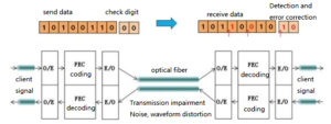
Рисунок 1: схематическая диаграмма функции FEC

Поэтому мы определяем FEC (упреждающая коррекция ошибок) как способность, которая гарантирует, что система связи все еще может обеспечивать безошибочную передачу под влиянием шума и других ухудшений. По сути, FEC представляет собой процесс кодирования и декодирования, а результат работы алгоритма отправляется в виде дополнительной информации вместе с данными от передатчика. Повторяя тот же алгоритм на дальнем конце, приемник может обнаруживать однобитовые ошибки и исправлять их (исправимые ошибки) без повторной передачи данных.

Чтобы измерить эту возможность, необходимо сосредоточиться на четырех параметрах FEC: допуске BER до коррекции, выигрыше кодирования (CG), служебной нагрузке (OH) и чистом выигрыше кодирования (NCG). Давайте взглянем на определение выигрыша кодирования NCG: оно определяет разницу между значением Q, соответствующим определенному уровню BER (например, 1 × 10-15), и значением Q (дБ), соответствующим уровню предварительной коррекции. BER толерантность.

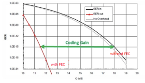
выигрыш от кодирования между определенным уровнем BEC с FEC и без FEC

Рисунок 2: выигрыш от кодирования между определенным уровнем BEC с FEC и без FEC

NCG можно сравнить с разницей в способности исправлять и получать правильную информацию между новичком и экспертом. Вообще говоря, существует два типа технологий FEC: внутриполосная FEC и внеполосная FEC.

Внутриполосный FEC: определяется стандартом ITU-T G.707. Он использует служебный байт кадра SDH для переноса символа FEC и в основном используется в системе SDH.
Внеполосный FEC: поддерживается стандартом ITU-T G.975/709. G.975 рекомендуется для FEC подводной оптической кабельной системы с использованием RS (255, 239), а G.709 модифицирован в соответствии с кодом FEC G.975.

В системе DWDM/OTN мы в основном используем внеполосную технологию FEC. В G.709 FEC Рида-Соломона (RS-FEC) определен для системы OTN, которая расположена в служебной части FEC уровня OTUk, и ее расположение показано на следующем рисунке.

расположение RS-FEC в G.709

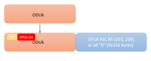
Рисунок 3: расположение RS-FEC в G.709

В настоящее время FEC разработана для многих поколений.

Первое поколение FEC в основном использует циклические коды или алгебраические коды, такие как коды RS (255, 239), определенные ITU-T G.975, которые часто называют стандартными FEC.
Второе поколение FEC в основном использует каскадные коды для построения FEC, такие как RS+RS или RS+BCH. Существует два типа FEC: расширенный FEC (EFEC) и дополнительный FEC (AFEC).
FEC третьего поколения использует мягкое решение или итерационные методы, такие как блочный турбокод и код проверки на четность с низкой плотностью LDPC.

Три поколения FEC

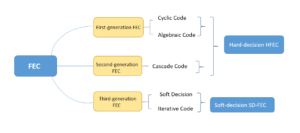
Рисунок 4: Три поколения FEC

В технологиях FEC первого и второго поколения при декодировании обычно используется только алгебраическая структура кода. Двоичная последовательность подается в декодер демодулятором, то есть демодулятор выполняет только решение 0, 1 по полученной последовательности. Этот метод декодирования называется Hard-Decision (HD-FEC). Различные виды жесткого решения FEC сравниваются следующим образом:

Кодирование	Алгоритм кодирования	Усиление кодирования	Линейная скорость	Стандарт
Внеполосный FEC	RS (255,239 XNUMX)	5 ~ 7dB	10.7Gbps	G.709
Расширенный FEC	RS (255,238 XNUMX) RS (245,210 XNUMX)	7 ~ 9dB	12.5Gbps	Нет
Advanced-FEC	RS (255,238 XNUMX) МПБ (900,860 XNUMX) МПБ (500,491 XNUMX)	7 ~ 9dB	10.7 Гбит / с.	G.709

Таблица XNUMX: Сравнение трех различных типов FEC с жестким решением

Мягкое решение, используемое в третьем поколении FEC (SD-FEC), представляет собой вероятностный метод декодирования. Он выполняет многобитовое квантование дискретизированного напряжения на выходе демодулятора, а затем отправляет его в декодер для декодирования алгебраической структуры кода.

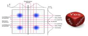
Принципиальная схема технологии мягких решений

Рисунок 5: Схематическая диаграмма технологии мягкого принятия решений

Как показано на рисунке выше, жесткое решение использует только одно пороговое значение для квантования одного бита, в то время как мягкое решение использует несколько пороговых значений для квантования восстановленных символов, получая однобитовую информацию плюс несколько битовую информацию о вероятности (достоверности). Это эквивалентно добавлению «Может быть» между «ДА» и «НЕТ». При том же коэффициенте накладных расходов усиление SD-FEC NCG на 1–1.5 дБ выше, чем у HFEC с жестким решением.

Накладные расходы	HD	SD	Дополнительный NCG (HD>SD)

0.07	10.00dB	11.10dB	1.10dB
0.15	10.95dB	12.20dB	1.25dB
0.25	11.60dB	12.90dB	1.30dB

Таблица XNUMX: сравнение NCG SD-FEC и HD-FEC

В настоящее время SD-FEC или гибридный метод кодирования, такой как SD-FEC и EFEC/HFEC, в основном используется в системах с разделением по длине волны 100G и выше. Взяв в качестве примера определение LDPC на конференции LOFC, его служебные данные и NCG показаны в следующей таблице.

Тип ФЭК	Оверхед ОН	NCG
EFEC+LDPC	0.205	10.8dB
LDPC	0.2	11.3dB
LDPC+СС	0.11	10.2dB
LDPC+СС	0.2	11.5dB
МПБ+LDPC	0.255	12.0dB

Таблица XNUMX: накладные расходы и NCG различных FEC

Из приведенной выше таблицы мы, кажется, выводим правило: чем выше служебная информация, используемая FEC, тем выше выигрыш от кодирования.

FEC подходит для высокоскоростной связи (25G, 40G и 100G, особенно 40G и 100G). Во время передачи оптический сигнал ухудшается из-за других факторов, что приводит к неправильной оценке на принимающей стороне. Он может ошибочно принять сигнал «1» за сигнал «0» или сигнал «0» за сигнал «1». Функция FEC формирует информационный код в код с возможностью исправления ошибок с помощью канального кодера на передающей стороне, а канальный декодер на принимающей стороне декодирует полученный код. Декодер обнаружит и исправит ошибку, чтобы улучшить качество сигнала, если количество ошибок, генерируемых при передаче, находится в пределах возможностей исправления ошибок (прерывистые ошибки).

Оптический модуль 100G QSFP28 и функция FEC

Функция FEC неизбежно вызовет некоторые задержки пакетов в процессе исправления битовых ошибок, поэтому не все 100G QSFP28 оптические модули должны включить эту функцию. Согласно стандартному протоколу IEEE, при использовании 100G QSFP28 LR4 оптический модуль, не рекомендуется включать FEC, и рекомендуется для других оптических модулей.

Оптические модули 100G QSFP28 разных компаний отличаются в некоторых аспектах. В следующей таблице показано, рекомендуется ли включать функцию FEC при использовании оптического модуля FiberMall 100G QSFP28.

Номер модели	Описание товара	С ФЭК
КСФП28-100Г-СР4	Модуль приемопередатчика 100G QSFP28 SR4 850nm 100m MTP/MPO MMF DDM	НЕТ
КСФП28-100Г-ЛР4	Модуль приемопередатчика 100G QSFP28 LR4 1310nm (LAN WDM) 10 км LC SMF DDM	НЕТ
КСФП28-100Г-ПСМ4	Модуль приемопередатчика 100G QSFP28 PSM4 1310nm 500m MTP/MPO SMF DDM	НЕТ
КСФП28-100Г-ИР4	Модуль приемопередатчика LC SMF DDM 100G QSFP28 IR4 1310nm (CWDM4) 2 км	Да
КСФП28-100Г-4ВДМ-10	Модуль приемопередатчика 100G QSFP28 4WDM 10 км LC SMF DDM	Да
КСФП28-100Г-ЭР4	Модуль приемопередатчика LC SMF DDM 100G QSFP28 ER4 Lite 1310nm (LAN WDM) 40 км	Да

Таблица четвертая: Вткак использовать FEC в FiberMall 100G QSFP28

Согласованность функций FEC на обоих концах канала

Функция FEC интерфейса является частью автосогласования. Когда на интерфейсе включено автосогласование, функция FEC определяется двумя концами канала посредством согласования. Если на одном конце включена функция FEC, на другом конце также должна быть включена функция FEC.

Стекирование и функция FEC

Если интерфейс настроен как физический порт-член стека, команда FEC не поддерживается. И наоборот, интерфейс, настроенный с помощью команды FEC, не может быть настроен как физический порт-член стека.

Сопутствующие товары:

How it worksEdit

ECC is accomplished by adding redundancy to the transmitted information using an algorithm. A redundant bit may be a complicated function of many original information bits. The original information may or may not appear literally in the encoded output; codes that include the unmodified input in the output are systematic, while those that do not are non-systematic.

A simplistic example of ECC is to transmit each data bit 3 times, which is known as a (3,1) repetition code. Through a noisy channel, a receiver might see 8 versions of the output, see table below.

Triplet received	Interpreted as
000	0 (error-free)
001	0
010	0
100	0
111	1 (error-free)
110	1
101	1
011	1

This allows an error in any one of the three samples to be corrected by «majority vote», or «democratic voting». The correcting ability of this ECC is:

Up to 1 bit of triplet in error, or
up to 2 bits of triplet omitted (cases not shown in table).

Though simple to implement and widely used, this triple modular redundancy is a relatively inefficient ECC. Better ECC codes typically examine the last several tens or even the last several hundreds of previously received bits to determine how to decode the current small handful of bits (typically in groups of 2 to 8 bits).

Averaging noise to reduce errorsEdit

ECC could be said to work by «averaging noise»; since each data bit affects many transmitted symbols, the corruption of some symbols by noise usually allows the original user data to be extracted from the other, uncorrupted received symbols that also depend on the same user data.

Because of this «risk-pooling» effect, digital communication systems that use ECC tend to work well above a certain minimum signal-to-noise ratio and not at all below it.
This all-or-nothing tendency – the cliff effect – becomes more pronounced as stronger codes are used that more closely approach the theoretical Shannon limit.
Interleaving ECC coded data can reduce the all or nothing properties of transmitted ECC codes when the channel errors tend to occur in bursts. However, this method has limits; it is best used on narrowband data.

Most telecommunication systems use a fixed channel code designed to tolerate the expected worst-case bit error rate, and then fail to work at all if the bit error rate is ever worse.
However, some systems adapt to the given channel error conditions: some instances of hybrid automatic repeat-request use a fixed ECC method as long as the ECC can handle the error rate, then switch to ARQ when the error rate gets too high;
adaptive modulation and coding uses a variety of ECC rates, adding more error-correction bits per packet when there are higher error rates in the channel, or taking them out when they are not needed.

Types of ECCEdit

A block code (specifically a Hamming code) where redundant bits are added as a block to the end of the initial message

A continuous code convolutional code where redundant bits are added continuously into the structure of the code word

The two main categories of ECC codes are block codes and convolutional codes.

Block codes work on fixed-size blocks (packets) of bits or symbols of predetermined size. Practical block codes can generally be hard-decoded in polynomial time to their block length.
Convolutional codes work on bit or symbol streams of arbitrary length. They are most often soft decoded with the Viterbi algorithm, though other algorithms are sometimes used. Viterbi decoding allows asymptotically optimal decoding efficiency with increasing constraint length of the convolutional code, but at the expense of exponentially increasing complexity. A convolutional code that is terminated is also a ‘block code’ in that it encodes a block of input data, but the block size of a convolutional code is generally arbitrary, while block codes have a fixed size dictated by their algebraic characteristics. Types of termination for convolutional codes include «tail-biting» and «bit-flushing».

There are many types of block codes; Reed–Solomon coding is noteworthy for its widespread use in compact discs, DVDs, and hard disk drives. Other examples of classical block codes include Golay, BCH, Multidimensional parity, and Hamming codes.

Hamming ECC is commonly used to correct NAND flash memory errors.^[6]
This provides single-bit error correction and 2-bit error detection.
Hamming codes are only suitable for more reliable single-level cell (SLC) NAND.
Denser multi-level cell (MLC) NAND may use multi-bit correcting ECC such as BCH or Reed–Solomon.^[7]^[8] NOR Flash typically does not use any error correction.^[7]

Classical block codes are usually decoded using hard-decision algorithms,^[9] which means that for every input and output signal a hard decision is made whether it corresponds to a one or a zero bit. In contrast, convolutional codes are typically decoded using soft-decision algorithms like the Viterbi, MAP or BCJR algorithms, which process (discretized) analog signals, and which allow for much higher error-correction performance than hard-decision decoding.

Nearly all classical block codes apply the algebraic properties of finite fields. Hence classical block codes are often referred to as algebraic codes.

In contrast to classical block codes that often specify an error-detecting or error-correcting ability, many modern block codes such as LDPC codes lack such guarantees. Instead, modern codes are evaluated in terms of their bit error rates.

Most forward error correction codes correct only bit-flips, but not bit-insertions or bit-deletions.
In this setting, the Hamming distance is the appropriate way to measure the bit error rate.
A few forward error correction codes are designed to correct bit-insertions and bit-deletions, such as Marker Codes and Watermark Codes.
The Levenshtein distance is a more appropriate way to measure the bit error rate when using such codes.
^[10]

Code-rate and the tradeoff between reliability and data rateEdit

The fundamental principle of ECC is to add redundant bits in order to help the decoder to find out the true message that was encoded by the transmitter. The code-rate of a given ECC system is defined as the ratio between the number of information bits and the total number of bits (i.e., information plus redundancy bits) in a given communication package. The code-rate is hence a real number. A low code-rate close to zero implies a strong code that uses many redundant bits to achieve a good performance, while a large code-rate close to 1 implies a weak code.

The redundant bits that protect the information have to be transferred using the same communication resources that they are trying to protect. This causes a fundamental tradeoff between reliability and data rate.^[11] In one extreme, a strong code (with low code-rate) can induce an important increase in the receiver SNR (signal-to-noise-ratio) decreasing the bit error rate, at the cost of reducing the effective data rate. On the other extreme, not using any ECC (i.e., a code-rate equal to 1) uses the full channel for information transfer purposes, at the cost of leaving the bits without any additional protection.

One interesting question is the following: how efficient in terms of information transfer can an ECC be that has a negligible decoding error rate? This question was answered by Claude Shannon with his second theorem, which says that the channel capacity is the maximum bit rate achievable by any ECC whose error rate tends to zero:^[12] His proof relies on Gaussian random coding, which is not suitable to real-world applications. The upper bound given by Shannon’s work inspired a long journey in designing ECCs that can come close to the ultimate performance boundary. Various codes today can attain almost the Shannon limit. However, capacity achieving ECCs are usually extremely complex to implement.

The most popular ECCs have a trade-off between performance and computational complexity. Usually, their parameters give a range of possible code rates, which can be optimized depending on the scenario. Usually, this optimization is done in order to achieve a low decoding error probability while minimizing the impact to the data rate. Another criterion for optimizing the code rate is to balance low error rate and retransmissions number in order to the energy cost of the communication.^[13]

Concatenated ECC codes for improved performanceEdit

Classical (algebraic) block codes and convolutional codes are frequently combined in concatenated coding schemes in which a short constraint-length Viterbi-decoded convolutional code does most of the work and a block code (usually Reed–Solomon) with larger symbol size and block length «mops up» any errors made by the convolutional decoder. Single pass decoding with this family of error correction codes can yield very low error rates, but for long range transmission conditions (like deep space) iterative decoding is recommended.

Concatenated codes have been standard practice in satellite and deep space communications since Voyager 2 first used the technique in its 1986 encounter with Uranus. The Galileo craft used iterative concatenated codes to compensate for the very high error rate conditions caused by having a failed antenna.

Low-density parity-check (LDPC)Edit

Low-density parity-check (LDPC) codes are a class of highly efficient linear block
codes made from many single parity check (SPC) codes. They can provide performance very close to the channel capacity (the theoretical maximum) using an iterated soft-decision decoding approach, at linear time complexity in terms of their block length. Practical implementations rely heavily on decoding the constituent SPC codes in parallel.

LDPC codes were first introduced by Robert G. Gallager in his PhD thesis in 1960,
but due to the computational effort in implementing encoder and decoder and the introduction of Reed–Solomon codes,
they were mostly ignored until the 1990s.

LDPC codes are now used in many recent high-speed communication standards, such as DVB-S2 (Digital Video Broadcasting – Satellite – Second Generation), WiMAX (IEEE 802.16e standard for microwave communications), High-Speed Wireless LAN (IEEE 802.11n),^[14] 10GBase-T Ethernet (802.3an) and G.hn/G.9960 (ITU-T Standard for networking over power lines, phone lines and coaxial cable). Other LDPC codes are standardized for wireless communication standards within 3GPP MBMS (see fountain codes).

Turbo codesEdit

Turbo coding is an iterated soft-decoding scheme that combines two or more relatively simple convolutional codes and an interleaver to produce a block code that can perform to within a fraction of a decibel of the Shannon limit. Predating LDPC codes in terms of practical application, they now provide similar performance.

One of the earliest commercial applications of turbo coding was the CDMA2000 1x (TIA IS-2000) digital cellular technology developed by Qualcomm and sold by Verizon Wireless, Sprint, and other carriers. It is also used for the evolution of CDMA2000 1x specifically for Internet access, 1xEV-DO (TIA IS-856). Like 1x, EV-DO was developed by Qualcomm, and is sold by Verizon Wireless, Sprint, and other carriers (Verizon’s marketing name for 1xEV-DO is Broadband Access, Sprint’s consumer and business marketing names for 1xEV-DO are Power Vision and Mobile Broadband, respectively).

Local decoding and testing of codesEdit

Sometimes it is only necessary to decode single bits of the message, or to check whether a given signal is a codeword, and do so without looking at the entire signal. This can make sense in a streaming setting, where codewords are too large to be classically decoded fast enough and where only a few bits of the message are of interest for now. Also such codes have become an important tool in computational complexity theory, e.g., for the design of probabilistically checkable proofs.

Locally decodable codes are error-correcting codes for which single bits of the message can be probabilistically recovered by only looking at a small (say constant) number of positions of a codeword, even after the codeword has been corrupted at some constant fraction of positions. Locally testable codes are error-correcting codes for which it can be checked probabilistically whether a signal is close to a codeword by only looking at a small number of positions of the signal.

InterleavingEdit

«Interleaver» redirects here. For the fiber-optic device, see optical interleaver.

A short illustration of interleaving idea

Interleaving is frequently used in digital communication and storage systems to improve the performance of forward error correcting codes. Many communication channels are not memoryless: errors typically occur in bursts rather than independently. If the number of errors within a code word exceeds the error-correcting code’s capability, it fails to recover the original code word. Interleaving alleviates this problem by shuffling source symbols across several code words, thereby creating a more uniform distribution of errors.^[15] Therefore, interleaving is widely used for burst error-correction.

The analysis of modern iterated codes, like turbo codes and LDPC codes, typically assumes an independent distribution of errors.^[16] Systems using LDPC codes therefore typically employ additional interleaving across the symbols within a code word.^[17]

For turbo codes, an interleaver is an integral component and its proper design is crucial for good performance.^[15]^[18] The iterative decoding algorithm works best when there are not short cycles in the factor graph that represents the decoder; the interleaver is chosen to avoid short cycles.

Interleaver designs include:

rectangular (or uniform) interleavers (similar to the method using skip factors described above)
convolutional interleavers
random interleavers (where the interleaver is a known random permutation)
S-random interleaver (where the interleaver is a known random permutation with the constraint that no input symbols within distance S appear within a distance of S in the output).^[19]
a contention-free quadratic permutation polynomial (QPP).^[20] An example of use is in the 3GPP Long Term Evolution mobile telecommunication standard.^[21]

In multi-carrier communication systems, interleaving across carriers may be employed to provide frequency diversity, e.g., to mitigate frequency-selective fading or narrowband interference.^[22]

ExampleEdit

Transmission without interleaving:

Error-free message:                                 aaaabbbbccccddddeeeeffffgggg
Transmission with a burst error:                    aaaabbbbccc____deeeeffffgggg

Here, each group of the same letter represents a 4-bit one-bit error-correcting codeword. The codeword cccc is altered in one bit and can be corrected, but the codeword dddd is altered in three bits, so either it cannot be decoded at all or it might be decoded incorrectly.

With interleaving:

Error-free code words:                              aaaabbbbccccddddeeeeffffgggg
Interleaved:                                        abcdefgabcdefgabcdefgabcdefg
Transmission with a burst error:                    abcdefgabcd____bcdefgabcdefg
Received code words after deinterleaving:           aa_abbbbccccdddde_eef_ffg_gg

In each of the codewords «aaaa», «eeee», «ffff», and «gggg», only one bit is altered, so one-bit error-correcting code will decode everything correctly.

Transmission without interleaving:

Original transmitted sentence:                      ThisIsAnExampleOfInterleaving
Received sentence with a burst error:               ThisIs______pleOfInterleaving

The term «AnExample» ends up mostly unintelligible and difficult to correct.

With interleaving:

Transmitted sentence:                               ThisIsAnExampleOfInterleaving...
Error-free transmission:                            TIEpfeaghsxlIrv.iAaenli.snmOten.
Received sentence with a burst error:               TIEpfe______Irv.iAaenli.snmOten.
Received sentence after deinterleaving:             T_isI_AnE_amp_eOfInterle_vin_...

No word is completely lost and the missing letters can be recovered with minimal guesswork.

Disadvantages of interleavingEdit

Use of interleaving techniques increases total delay. This is because the entire interleaved block must be received before the packets can be decoded.^[23] Also interleavers hide the structure of errors; without an interleaver, more advanced decoding algorithms can take advantage of the error structure and achieve more reliable communication than a simpler decoder combined with an interleaver^{[citation needed]}. An example of such an algorithm is based on neural network^[24] structures.

Software for error-correcting codesEdit

Simulating the behaviour of error-correcting codes (ECCs) in software is a common practice to design, validate and improve ECCs. The upcoming wireless 5G standard raises a new range of applications for the software ECCs: the Cloud Radio Access Networks (C-RAN) in a Software-defined radio (SDR) context. The idea is to directly use software ECCs in the communications. For instance in the 5G, the software ECCs could be located in the cloud and the antennas connected to this computing resources: improving this way the flexibility of the communication network and eventually increasing the energy efficiency of the system.

In this context, there are various available Open-source software listed below (non exhaustive).

AFF3CT(A Fast Forward Error Correction Toolbox): a full communication chain in C++ (many supported codes like Turbo, LDPC, Polar codes, etc.), very fast and specialized on channel coding (can be used as a program for simulations or as a library for the SDR).
IT++: a C++ library of classes and functions for linear algebra, numerical optimization, signal processing, communications, and statistics.
OpenAir: implementation (in C) of the 3GPP specifications concerning the Evolved Packet Core Networks.

List of error-correcting codesEdit

Distance	Code
2 (single-error detecting)	Parity
3 (single-error correcting)	Triple modular redundancy
3 (single-error correcting)	perfect Hamming such as Hamming(7,4)
4 (SECDED)	Extended Hamming
5 (double-error correcting)
6 (double-error correct-/triple error detect)	Nordstrom-Robinson code
7 (three-error correcting)	perfect binary Golay code
8 (TECFED)	extended binary Golay code

AN codes
Algebraic geometry code
BCH code, which can be designed to correct any arbitrary number of errors per code block.
Barker code used for radar, telemetry, ultra sound, Wifi, DSSS mobile phone networks, GPS etc.
Berger code
Constant-weight code
Convolutional code
Expander codes
Group codes
Golay codes, of which the Binary Golay code is of practical interest
Goppa code, used in the McEliece cryptosystem
Hadamard code
Hagelbarger code
Hamming code
Latin square based code for non-white noise (prevalent for example in broadband over powerlines)
Lexicographic code
Linear Network Coding, a type of erasure correcting code across networks instead of point-to-point links
Long code
Low-density parity-check code, also known as Gallager code, as the archetype for sparse graph codes
LT code, which is a near-optimal rateless erasure correcting code (Fountain code)
m of n codes
Nordstrom-Robinson code, used in Geometry and Group Theory^[25]
Online code, a near-optimal rateless erasure correcting code
Polar code (coding theory)
Raptor code, a near-optimal rateless erasure correcting code
Reed–Solomon error correction
Reed–Muller code
Repeat-accumulate code
Repetition codes, such as Triple modular redundancy
Spinal code, a rateless, nonlinear code based on pseudo-random hash functions^[26]
Tornado code, a near-optimal erasure correcting code, and the precursor to Fountain codes
Turbo code
Walsh–Hadamard code
Cyclic redundancy checks (CRCs) can correct 1-bit errors for messages at most bits long for optimal generator polynomials of degree , see Mathematics of cyclic redundancy checks#Bitfilters

ReferencesEdit

^ Charles Wang; Dean Sklar; Diana Johnson (Winter 2001–2002). «Forward Error-Correction Coding». Crosslink. The Aerospace Corporation. 3 (1). Archived from the original on 14 March 2012. Retrieved 5 March 2006.
^ Charles Wang; Dean Sklar; Diana Johnson (Winter 2001–2002). «Forward Error-Correction Coding». Crosslink. The Aerospace Corporation. 3 (1). Archived from the original on 14 March 2012. Retrieved 5 March 2006. How Forward Error-Correcting Codes Work]
^ ^a ^b Maunder, Robert (2016). «Overview of Channel Coding».
^ Glover, Neal; Dudley, Trent (1990). Practical Error Correction Design For Engineers (Revision 1.1, 2nd ed.). CO, USA: Cirrus Logic. ISBN 0-927239-00-0.
^ ^a ^b Hamming, Richard Wesley (April 1950). «Error Detecting and Error Correcting Codes». Bell System Technical Journal. USA: AT&T. 29 (2): 147–160. doi:10.1002/j.1538-7305.1950.tb00463.x. S2CID 61141773.
^ «Hamming codes for NAND flash memory devices» Archived 21 August 2016 at the Wayback Machine. EE Times-Asia. Apparently based on «Micron Technical Note TN-29-08: Hamming Codes for NAND Flash Memory Devices». 2005. Both say: «The Hamming algorithm is an industry-accepted method for error detection and correction in many SLC NAND flash-based applications.»
^ ^a ^b «What Types of ECC Should Be Used on Flash Memory?» (Application note). Spansion. 2011. Both Reed–Solomon algorithm and BCH algorithm are common ECC choices for MLC NAND flash. … Hamming based block codes are the most commonly used ECC for SLC…. both Reed–Solomon and BCH are able to handle multiple errors and are widely used on MLC flash.
^ Jim Cooke (August 2007). «The Inconvenient Truths of NAND Flash Memory» (PDF). p. 28. For SLC, a code with a correction threshold of 1 is sufficient. t=4 required … for MLC.
^ Baldi, M.; Chiaraluce, F. (2008). «A Simple Scheme for Belief Propagation Decoding of BCH and RS Codes in Multimedia Transmissions». International Journal of Digital Multimedia Broadcasting. 2008: 1–12. doi:10.1155/2008/957846.
^ Shah, Gaurav; Molina, Andres; Blaze, Matt (2006). «Keyboards and covert channels». USENIX. Retrieved 20 December 2018.
^ Tse, David; Viswanath, Pramod (2005), Fundamentals of Wireless Communication, Cambridge University Press, UK
^ Shannon, C. E. (1948). «A mathematical theory of communication» (PDF). Bell System Technical Journal. 27 (3–4): 379–423 & 623–656. doi:10.1002/j.1538-7305.1948.tb01338.x. hdl:11858/00-001M-0000-002C-4314-2.
^ Rosas, F.; Brante, G.; Souza, R. D.; Oberli, C. (2014). «Optimizing the code rate for achieving energy-efficient wireless communications». Proceedings of the IEEE Wireless Communications and Networking Conference (WCNC). pp. 775–780. doi:10.1109/WCNC.2014.6952166. ISBN 978-1-4799-3083-8.
^ IEEE Standard, section 20.3.11.6 «802.11n-2009» Archived 3 February 2013 at the Wayback Machine, IEEE, 29 October 2009, accessed 21 March 2011.
^ ^a ^b Vucetic, B.; Yuan, J. (2000). Turbo codes: principles and applications. Springer Verlag. ISBN 978-0-7923-7868-6.
^ Luby, Michael; Mitzenmacher, M.; Shokrollahi, A.; Spielman, D.; Stemann, V. (1997). «Practical Loss-Resilient Codes». Proc. 29th Annual Association for Computing Machinery (ACM) Symposium on Theory of Computation.
^ «Digital Video Broadcast (DVB); Second generation framing structure, channel coding and modulation systems for Broadcasting, Interactive Services, News Gathering and other satellite broadband applications (DVB-S2)». En 302 307. ETSI (V1.2.1). April 2009.
^ Andrews, K. S.; Divsalar, D.; Dolinar, S.; Hamkins, J.; Jones, C. R.; Pollara, F. (November 2007). «The Development of Turbo and LDPC Codes for Deep-Space Applications». Proceedings of the IEEE. 95 (11): 2142–2156. doi:10.1109/JPROC.2007.905132. S2CID 9289140.
^ Dolinar, S.; Divsalar, D. (15 August 1995). «Weight Distributions for Turbo Codes Using Random and Nonrandom Permutations». TDA Progress Report. 122: 42–122. Bibcode:1995TDAPR.122…56D. CiteSeerX 10.1.1.105.6640.
^ Takeshita, Oscar (2006). «Permutation Polynomial Interleavers: An Algebraic-Geometric Perspective». IEEE Transactions on Information Theory. 53 (6): 2116–2132. arXiv:cs/0601048. Bibcode:2006cs……..1048T. doi:10.1109/TIT.2007.896870. S2CID 660.
^ 3GPP TS 36.212, version 8.8.0, page 14
^ «Digital Video Broadcast (DVB); Frame structure, channel coding and modulation for a second generation digital terrestrial television broadcasting system (DVB-T2)». En 302 755. ETSI (V1.1.1). September 2009.
^ Techie (3 June 2010). «Explaining Interleaving». W3 Techie Blog. Retrieved 3 June 2010.
^ Krastanov, Stefan; Jiang, Liang (8 September 2017). «Deep Neural Network Probabilistic Decoder for Stabilizer Codes». Scientific Reports. 7 (1): 11003. arXiv:1705.09334. Bibcode:2017NatSR…711003K. doi:10.1038/s41598-017-11266-1. PMC 5591216. PMID 28887480.
^ Nordstrom, A.W.; Robinson, J.P. (1967), «An optimum nonlinear code», Information and Control, 11 (5–6): 613–616, doi:10.1016/S0019-9958(67)90835-2
^ Perry, Jonathan; Balakrishnan, Hari; Shah, Devavrat (2011). «Rateless Spinal Codes». Proceedings of the 10th ACM Workshop on Hot Topics in Networks. pp. 1–6. doi:10.1145/2070562.2070568. hdl:1721.1/79676. ISBN 9781450310598.

External linksEdit

Morelos-Zaragoza, Robert (2004). «The Correcting Codes (ECC) Page». Retrieved 5 March 2006.
lpdec: library for LP decoding and related things (Python)

Источник

Что такое FEC?

Каковы типы и особенности FEC?

Типы

Характеристики

Применение FEC в 100G сетях

Замечания для FEC в сетях 100G

Метод реализации

Поддерживает ли коммутатор FEC

Включить ли FEC на QSFP28 100G модулях

Согласованность функций FEC на обоих концах канала

Стекирование & FEC

Заключение

High-capacity long-haul optical fiber transmission

8.4.4 Capacity-approaching FEC

Ultralong-distance undersea transmission systems

13.2.3.1 Adaptive rate forward error correction

Technique Developments and Market Prospects of Submarine Optical Cable Engineering

10.1.2 Development Trends of the Forward Error Correction Technique

Communicating pictures: delivery across networks

Cross-packet FEC

Error-Resilience Video Coding Techniques

9.6.1 Forward Error Correction (FEC)

Applications to Communication Systems

6.2.2 Recent Trends in Operational Systems

50-Gb/s passive optical network (50G-PON)

10.3.1 LDPC design considerations and performances

Coding and Error Correction in Optical Fiber Communications Systems

3.4 Potential Role of Forward Error-Correcting Codes in Fiber Systems and Its Beneficial Ripple Effects on System and Hardware Designs

Video Transmission over Networks

Transport-Level Error Control

Forward Error Control Coding

Automatic Repeat Request

Classical Error Correcting Codes

6.6 Concluding Remarks

Оптический модуль 100G QSFP28 и функция FEC

Согласованность функций FEC на обоих концах канала

Стекирование и функция FEC

Сопутствующие товары:

Похожие посты:

How it worksEdit

Averaging noise to reduce errorsEdit

Types of ECCEdit

Code-rate and the tradeoff between reliability and data rateEdit

Concatenated ECC codes for improved performanceEdit

Low-density parity-check (LDPC)Edit

Turbo codesEdit

Local decoding and testing of codesEdit

InterleavingEdit

ExampleEdit

Disadvantages of interleavingEdit

Software for error-correcting codesEdit

List of error-correcting codesEdit

See alsoEdit

ReferencesEdit

Further readingEdit

External linksEdit