From Wikipedia, the free encyclopedia
In statistics, the mean squared error (MSE)[1] or mean squared deviation (MSD) of an estimator (of a procedure for estimating an unobserved quantity) measures the average of the squares of the errors—that is, the average squared difference between the estimated values and the actual value. MSE is a risk function, corresponding to the expected value of the squared error loss.[2] The fact that MSE is almost always strictly positive (and not zero) is because of randomness or because the estimator does not account for information that could produce a more accurate estimate.[3] In machine learning, specifically empirical risk minimization, MSE may refer to the empirical risk (the average loss on an observed data set), as an estimate of the true MSE (the true risk: the average loss on the actual population distribution).
The MSE is a measure of the quality of an estimator. As it is derived from the square of Euclidean distance, it is always a positive value that decreases as the error approaches zero.
The MSE is the second moment (about the origin) of the error, and thus incorporates both the variance of the estimator (how widely spread the estimates are from one data sample to another) and its bias (how far off the average estimated value is from the true value).[citation needed] For an unbiased estimator, the MSE is the variance of the estimator. Like the variance, MSE has the same units of measurement as the square of the quantity being estimated. In an analogy to standard deviation, taking the square root of MSE yields the root-mean-square error or root-mean-square deviation (RMSE or RMSD), which has the same units as the quantity being estimated; for an unbiased estimator, the RMSE is the square root of the variance, known as the standard error.
Definition and basic properties[edit]
The MSE either assesses the quality of a predictor (i.e., a function mapping arbitrary inputs to a sample of values of some random variable), or of an estimator (i.e., a mathematical function mapping a sample of data to an estimate of a parameter of the population from which the data is sampled). The definition of an MSE differs according to whether one is describing a predictor or an estimator.
Predictor[edit]
If a vector of 


In other words, the MSE is the mean 

In matrix notation,

where 


The MSE can also be computed on q data points that were not used in estimating the model, either because they were held back for this purpose, or because these data have been newly obtained. Within this process, known as statistical learning, the MSE is often called the test MSE,[4] and is computed as

Estimator[edit]
The MSE of an estimator 

![{displaystyle operatorname {MSE} ({hat {theta }})=operatorname {E} _{theta }left[({hat {theta }}-theta )^{2}right].}](https://wikimedia.org/api/rest_v1/media/math/render/svg/9a0e1b3bac58f9ba2d2f4ff8b85b2e35a8f4bf78)
This definition depends on the unknown parameter, but the MSE is a priori a property of an estimator. The MSE could be a function of unknown parameters, in which case any estimator of the MSE based on estimates of these parameters would be a function of the data (and thus a random variable). If the estimator
The MSE can be written as the sum of the variance of the estimator and the squared bias of the estimator, providing a useful way to calculate the MSE and implying that in the case of unbiased estimators, the MSE and variance are equivalent.[5]

Proof of variance and bias relationship[edit]
![{displaystyle {begin{aligned}operatorname {MSE} ({hat {theta }})&=operatorname {E} _{theta }left[({hat {theta }}-theta )^{2}right]\&=operatorname {E} _{theta }left[left({hat {theta }}-operatorname {E} _{theta }[{hat {theta }}]+operatorname {E} _{theta }[{hat {theta }}]-theta right)^{2}right]\&=operatorname {E} _{theta }left[left({hat {theta }}-operatorname {E} _{theta }[{hat {theta }}]right)^{2}+2left({hat {theta }}-operatorname {E} _{theta }[{hat {theta }}]right)left(operatorname {E} _{theta }[{hat {theta }}]-theta right)+left(operatorname {E} _{theta }[{hat {theta }}]-theta right)^{2}right]\&=operatorname {E} _{theta }left[left({hat {theta }}-operatorname {E} _{theta }[{hat {theta }}]right)^{2}right]+operatorname {E} _{theta }left[2left({hat {theta }}-operatorname {E} _{theta }[{hat {theta }}]right)left(operatorname {E} _{theta }[{hat {theta }}]-theta right)right]+operatorname {E} _{theta }left[left(operatorname {E} _{theta }[{hat {theta }}]-theta right)^{2}right]\&=operatorname {E} _{theta }left[left({hat {theta }}-operatorname {E} _{theta }[{hat {theta }}]right)^{2}right]+2left(operatorname {E} _{theta }[{hat {theta }}]-theta right)operatorname {E} _{theta }left[{hat {theta }}-operatorname {E} _{theta }[{hat {theta }}]right]+left(operatorname {E} _{theta }[{hat {theta }}]-theta right)^{2}&&operatorname {E} _{theta }[{hat {theta }}]-theta ={text{const.}}\&=operatorname {E} _{theta }left[left({hat {theta }}-operatorname {E} _{theta }[{hat {theta }}]right)^{2}right]+2left(operatorname {E} _{theta }[{hat {theta }}]-theta right)left(operatorname {E} _{theta }[{hat {theta }}]-operatorname {E} _{theta }[{hat {theta }}]right)+left(operatorname {E} _{theta }[{hat {theta }}]-theta right)^{2}&&operatorname {E} _{theta }[{hat {theta }}]={text{const.}}\&=operatorname {E} _{theta }left[left({hat {theta }}-operatorname {E} _{theta }[{hat {theta }}]right)^{2}right]+left(operatorname {E} _{theta }[{hat {theta }}]-theta right)^{2}\&=operatorname {Var} _{theta }({hat {theta }})+operatorname {Bias} _{theta }({hat {theta }},theta )^{2}end{aligned}}}](https://wikimedia.org/api/rest_v1/media/math/render/svg/2ac524a751828f971013e1297a33ca1cc4c38cd6)
An even shorter proof can be achieved using the well-known formula that for a random variable 


![{displaystyle {begin{aligned}operatorname {MSE} ({hat {theta }})&=mathbb {E} [({hat {theta }}-theta )^{2}]\&=operatorname {Var} ({hat {theta }}-theta )+(mathbb {E} [{hat {theta }}-theta ])^{2}\&=operatorname {Var} ({hat {theta }})+operatorname {Bias} ^{2}({hat {theta }})end{aligned}}}](https://wikimedia.org/api/rest_v1/media/math/render/svg/864646cf4426e2b62a3caf9460382eec1a77fe4e)
But in real modeling case, MSE could be described as the addition of model variance, model bias, and irreducible uncertainty (see Bias–variance tradeoff). According to the relationship, the MSE of the estimators could be simply used for the efficiency comparison, which includes the information of estimator variance and bias. This is called MSE criterion.
In regression[edit]
In regression analysis, plotting is a more natural way to view the overall trend of the whole data. The mean of the distance from each point to the predicted regression model can be calculated, and shown as the mean squared error. The squaring is critical to reduce the complexity with negative signs. To minimize MSE, the model could be more accurate, which would mean the model is closer to actual data. One example of a linear regression using this method is the least squares method—which evaluates appropriateness of linear regression model to model bivariate dataset,[6] but whose limitation is related to known distribution of the data.
The term mean squared error is sometimes used to refer to the unbiased estimate of error variance: the residual sum of squares divided by the number of degrees of freedom. This definition for a known, computed quantity differs from the above definition for the computed MSE of a predictor, in that a different denominator is used. The denominator is the sample size reduced by the number of model parameters estimated from the same data, (n−p) for p regressors or (n−p−1) if an intercept is used (see errors and residuals in statistics for more details).[7] Although the MSE (as defined in this article) is not an unbiased estimator of the error variance, it is consistent, given the consistency of the predictor.
In regression analysis, «mean squared error», often referred to as mean squared prediction error or «out-of-sample mean squared error», can also refer to the mean value of the squared deviations of the predictions from the true values, over an out-of-sample test space, generated by a model estimated over a particular sample space. This also is a known, computed quantity, and it varies by sample and by out-of-sample test space.
Examples[edit]
Mean[edit]
Suppose we have a random sample of size 


which has an expected value equal to the true mean
![{displaystyle operatorname {MSE} left({overline {X}}right)=operatorname {E} left[left({overline {X}}-mu right)^{2}right]=left({frac {sigma }{sqrt {n}}}right)^{2}={frac {sigma ^{2}}{n}}}](https://wikimedia.org/api/rest_v1/media/math/render/svg/b4647a2cc4c8f9a4c90b628faad2dcf80c4aae84)
where 
For a Gaussian distribution, this is the best unbiased estimator (i.e., one with the lowest MSE among all unbiased estimators), but not, say, for a uniform distribution.
Variance[edit]
The usual estimator for the variance is the corrected sample variance:

This is unbiased (its expected value is

where 

However, one can use other estimators for 

then we calculate:
![{displaystyle {begin{aligned}operatorname {MSE} (S_{a}^{2})&=operatorname {E} left[left({frac {n-1}{a}}S_{n-1}^{2}-sigma ^{2}right)^{2}right]\&=operatorname {E} left[{frac {(n-1)^{2}}{a^{2}}}S_{n-1}^{4}-2left({frac {n-1}{a}}S_{n-1}^{2}right)sigma ^{2}+sigma ^{4}right]\&={frac {(n-1)^{2}}{a^{2}}}operatorname {E} left[S_{n-1}^{4}right]-2left({frac {n-1}{a}}right)operatorname {E} left[S_{n-1}^{2}right]sigma ^{2}+sigma ^{4}\&={frac {(n-1)^{2}}{a^{2}}}operatorname {E} left[S_{n-1}^{4}right]-2left({frac {n-1}{a}}right)sigma ^{4}+sigma ^{4}&&operatorname {E} left[S_{n-1}^{2}right]=sigma ^{2}\&={frac {(n-1)^{2}}{a^{2}}}left({frac {gamma _{2}}{n}}+{frac {n+1}{n-1}}right)sigma ^{4}-2left({frac {n-1}{a}}right)sigma ^{4}+sigma ^{4}&&operatorname {E} left[S_{n-1}^{4}right]=operatorname {MSE} (S_{n-1}^{2})+sigma ^{4}\&={frac {n-1}{na^{2}}}left((n-1)gamma _{2}+n^{2}+nright)sigma ^{4}-2left({frac {n-1}{a}}right)sigma ^{4}+sigma ^{4}end{aligned}}}](https://wikimedia.org/api/rest_v1/media/math/render/svg/cf22322412b8454c706d78671e5d94208675a6e0)
This is minimized when

For a Gaussian distribution, where 


Further, while the corrected sample variance is the best unbiased estimator (minimum mean squared error among unbiased estimators) of variance for Gaussian distributions, if the distribution is not Gaussian, then even among unbiased estimators, the best unbiased estimator of the variance may not be 
Gaussian distribution[edit]
The following table gives several estimators of the true parameters of the population, μ and σ2, for the Gaussian case.[9]
| True value | Estimator | Mean squared error |
|---|---|---|
 |
= the unbiased estimator of the population mean,  |

|
 |
= the unbiased estimator of the population variance,  |

|
|
= the biased estimator of the population variance,  |

|
|
= the biased estimator of the population variance,  |

|
Interpretation[edit]
An MSE of zero, meaning that the estimator
Values of MSE may be used for comparative purposes. Two or more statistical models may be compared using their MSEs—as a measure of how well they explain a given set of observations: An unbiased estimator (estimated from a statistical model) with the smallest variance among all unbiased estimators is the best unbiased estimator or MVUE (Minimum-Variance Unbiased Estimator).
Both analysis of variance and linear regression techniques estimate the MSE as part of the analysis and use the estimated MSE to determine the statistical significance of the factors or predictors under study. The goal of experimental design is to construct experiments in such a way that when the observations are analyzed, the MSE is close to zero relative to the magnitude of at least one of the estimated treatment effects.
In one-way analysis of variance, MSE can be calculated by the division of the sum of squared errors and the degree of freedom. Also, the f-value is the ratio of the mean squared treatment and the MSE.
MSE is also used in several stepwise regression techniques as part of the determination as to how many predictors from a candidate set to include in a model for a given set of observations.
Applications[edit]
- Minimizing MSE is a key criterion in selecting estimators: see minimum mean-square error. Among unbiased estimators, minimizing the MSE is equivalent to minimizing the variance, and the estimator that does this is the minimum variance unbiased estimator. However, a biased estimator may have lower MSE; see estimator bias.
- In statistical modelling the MSE can represent the difference between the actual observations and the observation values predicted by the model. In this context, it is used to determine the extent to which the model fits the data as well as whether removing some explanatory variables is possible without significantly harming the model’s predictive ability.
- In forecasting and prediction, the Brier score is a measure of forecast skill based on MSE.
Loss function[edit]
Squared error loss is one of the most widely used loss functions in statistics[citation needed], though its widespread use stems more from mathematical convenience than considerations of actual loss in applications. Carl Friedrich Gauss, who introduced the use of mean squared error, was aware of its arbitrariness and was in agreement with objections to it on these grounds.[3] The mathematical benefits of mean squared error are particularly evident in its use at analyzing the performance of linear regression, as it allows one to partition the variation in a dataset into variation explained by the model and variation explained by randomness.
Criticism[edit]
The use of mean squared error without question has been criticized by the decision theorist James Berger. Mean squared error is the negative of the expected value of one specific utility function, the quadratic utility function, which may not be the appropriate utility function to use under a given set of circumstances. There are, however, some scenarios where mean squared error can serve as a good approximation to a loss function occurring naturally in an application.[10]
Like variance, mean squared error has the disadvantage of heavily weighting outliers.[11] This is a result of the squaring of each term, which effectively weights large errors more heavily than small ones. This property, undesirable in many applications, has led researchers to use alternatives such as the mean absolute error, or those based on the median.
See also[edit]
- Bias–variance tradeoff
- Hodges’ estimator
- James–Stein estimator
- Mean percentage error
- Mean square quantization error
- Mean square weighted deviation
- Mean squared displacement
- Mean squared prediction error
- Minimum mean square error
- Minimum mean squared error estimator
- Overfitting
- Peak signal-to-noise ratio
Notes[edit]
- ^ This can be proved by Jensen’s inequality as follows. The fourth central moment is an upper bound for the square of variance, so that the least value for their ratio is one, therefore, the least value for the excess kurtosis is −2, achieved, for instance, by a Bernoulli with p=1/2.
References[edit]
- ^ a b «Mean Squared Error (MSE)». www.probabilitycourse.com. Retrieved 2020-09-12.
- ^ Bickel, Peter J.; Doksum, Kjell A. (2015). Mathematical Statistics: Basic Ideas and Selected Topics. Vol. I (Second ed.). p. 20.
If we use quadratic loss, our risk function is called the mean squared error (MSE) …
- ^ a b Lehmann, E. L.; Casella, George (1998). Theory of Point Estimation (2nd ed.). New York: Springer. ISBN 978-0-387-98502-2. MR 1639875.
- ^ Gareth, James; Witten, Daniela; Hastie, Trevor; Tibshirani, Rob (2021). An Introduction to Statistical Learning: with Applications in R. Springer. ISBN 978-1071614174.
- ^ Wackerly, Dennis; Mendenhall, William; Scheaffer, Richard L. (2008). Mathematical Statistics with Applications (7 ed.). Belmont, CA, USA: Thomson Higher Education. ISBN 978-0-495-38508-0.
- ^ A modern introduction to probability and statistics : understanding why and how. Dekking, Michel, 1946-. London: Springer. 2005. ISBN 978-1-85233-896-1. OCLC 262680588.
{{cite book}}: CS1 maint: others (link) - ^ Steel, R.G.D, and Torrie, J. H., Principles and Procedures of Statistics with Special Reference to the Biological Sciences., McGraw Hill, 1960, page 288.
- ^ Mood, A.; Graybill, F.; Boes, D. (1974). Introduction to the Theory of Statistics (3rd ed.). McGraw-Hill. p. 229.
- ^ DeGroot, Morris H. (1980). Probability and Statistics (2nd ed.). Addison-Wesley.
- ^ Berger, James O. (1985). «2.4.2 Certain Standard Loss Functions». Statistical Decision Theory and Bayesian Analysis (2nd ed.). New York: Springer-Verlag. p. 60. ISBN 978-0-387-96098-2. MR 0804611.
- ^ Bermejo, Sergio; Cabestany, Joan (2001). «Oriented principal component analysis for large margin classifiers». Neural Networks. 14 (10): 1447–1461. doi:10.1016/S0893-6080(01)00106-X. PMID 11771723.
17 авг. 2022 г.
читать 3 мин
В статистике регрессионный анализ — это метод, который мы используем для понимания взаимосвязи между переменной-предиктором x и переменной отклика y.
Когда мы проводим регрессионный анализ, мы получаем модель, которая сообщает нам прогнозируемое значение для переменной ответа на основе значения переменной-предиктора.
Один из способов оценить, насколько «хорошо» наша модель соответствует заданному набору данных, — это вычислить среднеквадратичную ошибку , которая представляет собой показатель, который говорит нам, насколько в среднем наши прогнозируемые значения отличаются от наших наблюдаемых значений.
Формула для нахождения среднеквадратичной ошибки, чаще называемая RMSE , выглядит следующим образом:
СКО = √[ Σ(P i – O i ) 2 / n ]
куда:
- Σ — причудливый символ, означающий «сумма».
- P i — прогнозируемое значение для i -го наблюдения в наборе данных.
- O i — наблюдаемое значение для i -го наблюдения в наборе данных.
- n — размер выборки
Технические примечания:
- Среднеквадратичную ошибку можно рассчитать для любого типа модели, которая дает прогнозные значения, которые затем можно сравнить с наблюдаемыми значениями набора данных.
- Среднеквадратичную ошибку также иногда называют среднеквадратичным отклонением, которое часто обозначается аббревиатурой RMSD.
Далее рассмотрим пример расчета среднеквадратичной ошибки в Excel.
Как рассчитать среднеквадратичную ошибку в Excel
В Excel нет встроенной функции для расчета RMSE, но мы можем довольно легко вычислить его с помощью одной формулы. Мы покажем, как рассчитать RMSE для двух разных сценариев.
Сценарий 1
В одном сценарии у вас может быть один столбец, содержащий предсказанные значения вашей модели, и другой столбец, содержащий наблюдаемые значения. На изображении ниже показан пример такого сценария:

Если это так, то вы можете рассчитать RMSE, введя следующую формулу в любую ячейку, а затем нажав CTRL+SHIFT+ENTER:
=КОРЕНЬ(СУММСК(A2:A21-B2:B21) / СЧЕТЧ(A2:A21))
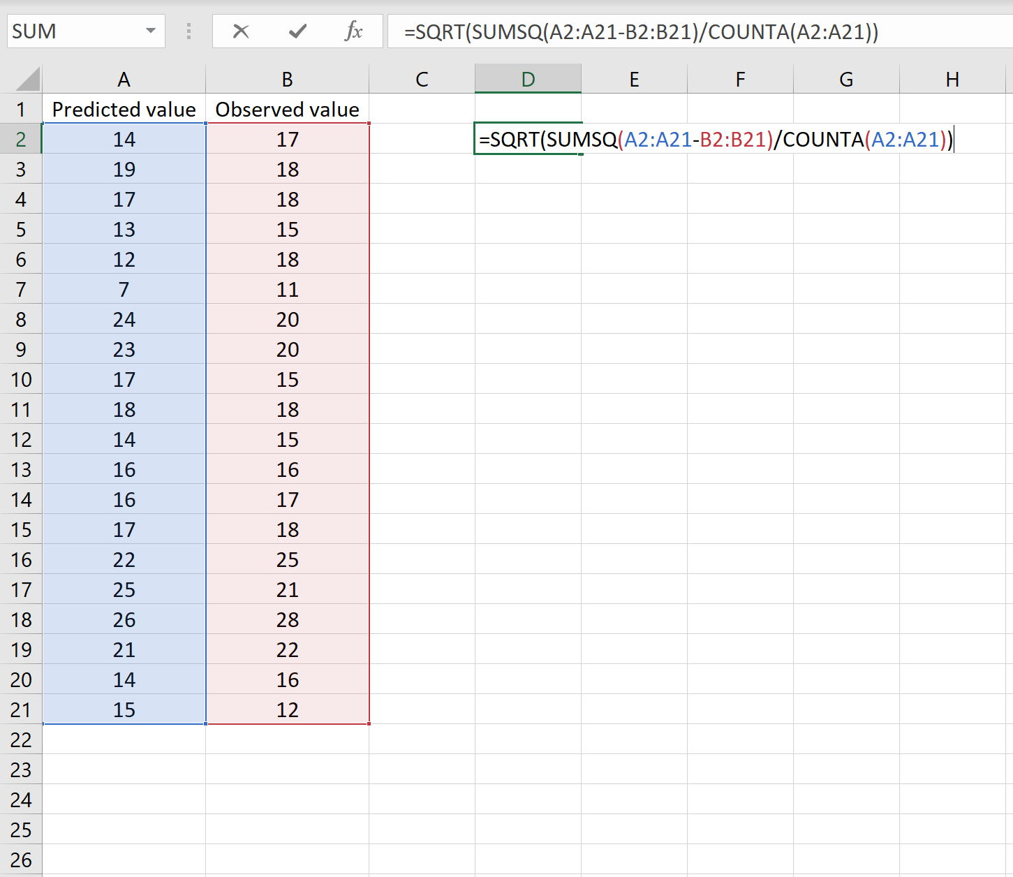
Это говорит нам о том, что среднеквадратическая ошибка равна 2,6646 .
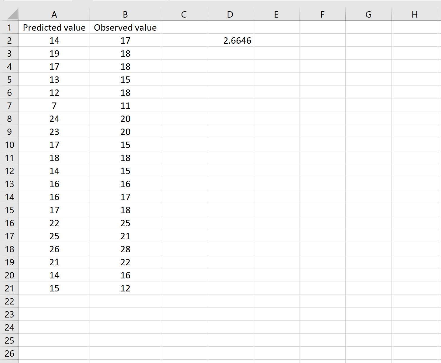
Формула может показаться немного сложной, но она имеет смысл, если ее разобрать:
= КОРЕНЬ( СУММСК(A2:A21-B2:B21) / СЧЕТЧ(A2:A21) )
- Во-первых, мы вычисляем сумму квадратов разностей между прогнозируемыми и наблюдаемыми значениями, используя функцию СУММСК() .
- Затем мы делим на размер выборки набора данных, используя COUNTA() , который подсчитывает количество непустых ячеек в диапазоне.
- Наконец, мы извлекаем квадратный корень из всего вычисления, используя функцию SQRT() .
Сценарий 2
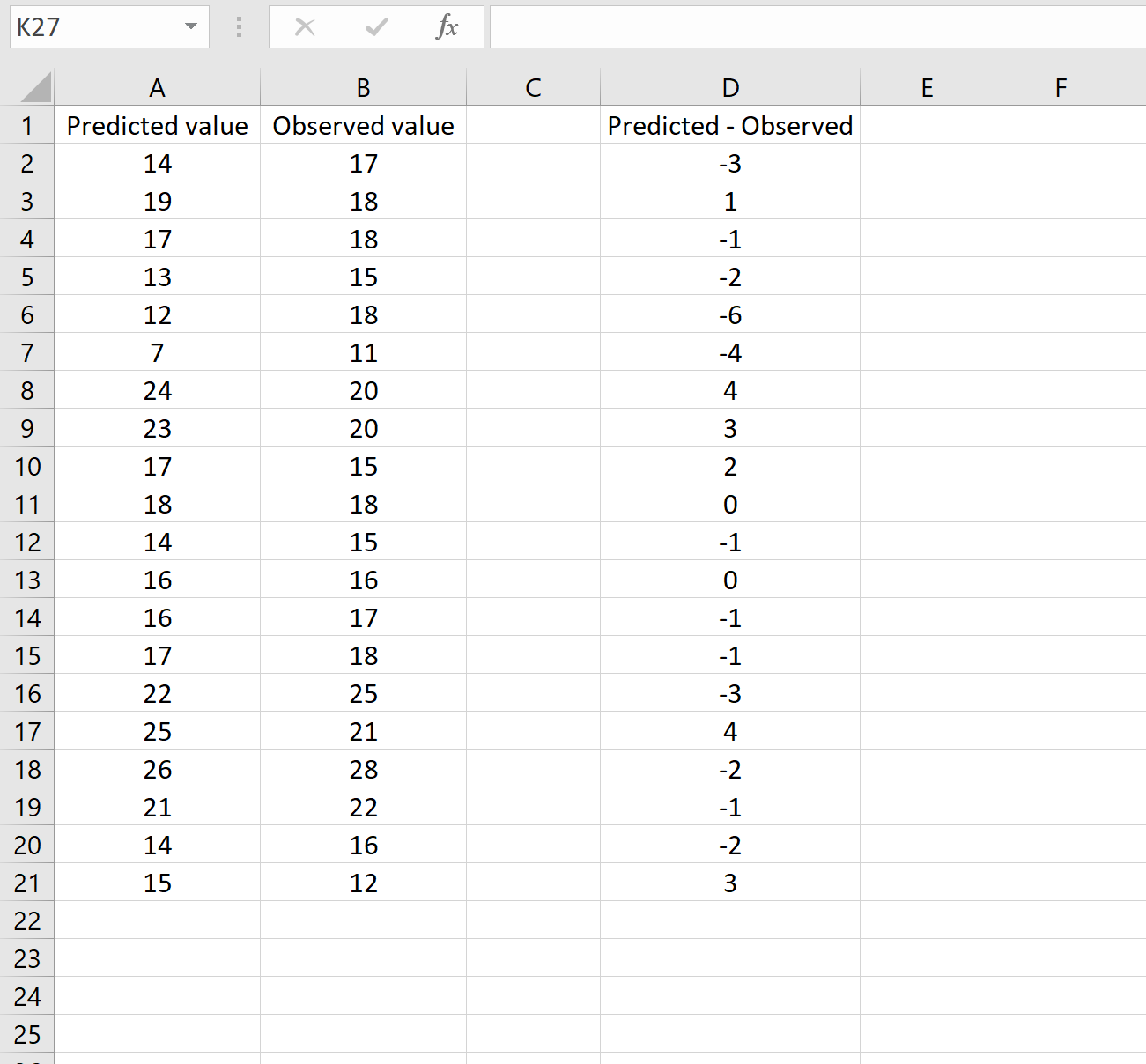
В другом сценарии вы, возможно, уже вычислили разницу между прогнозируемыми и наблюдаемыми значениями. В этом случае у вас будет только один столбец, отображающий различия.
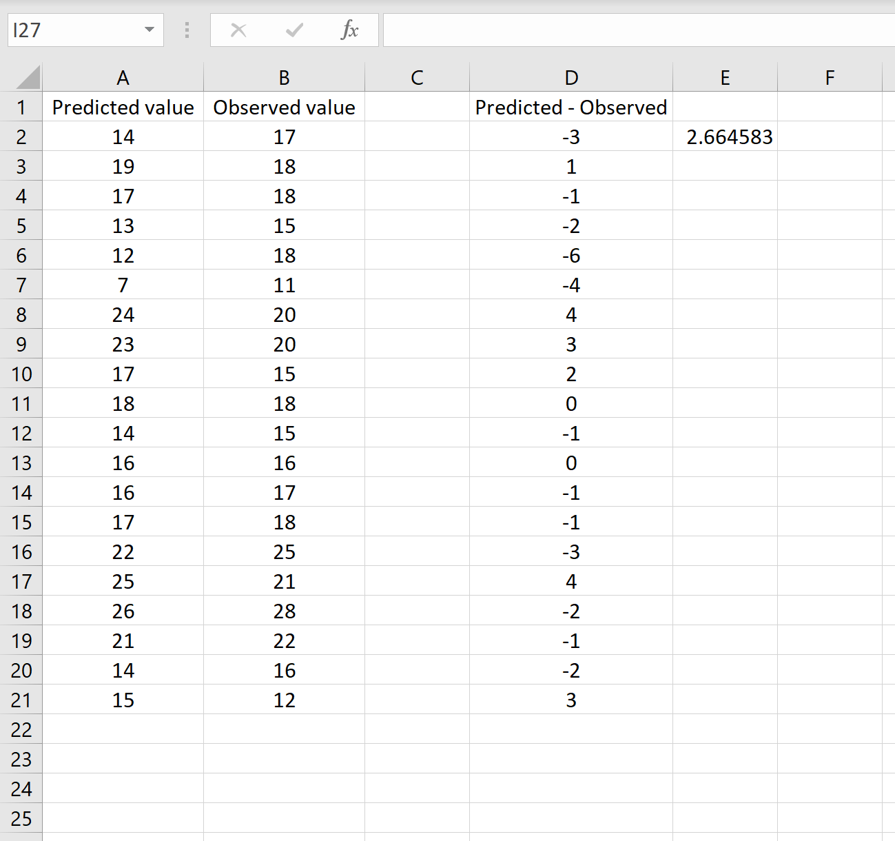
На изображении ниже показан пример этого сценария. Прогнозируемые значения отображаются в столбце A, наблюдаемые значения — в столбце B, а разница между прогнозируемыми и наблюдаемыми значениями — в столбце D:
Если это так, то вы можете рассчитать RMSE, введя следующую формулу в любую ячейку, а затем нажав CTRL+SHIFT+ENTER:
=КОРЕНЬ(СУММСК(D2:D21) / СЧЕТЧ(D2:D21))
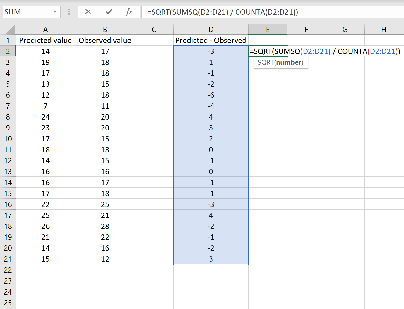
Это говорит нам о том, что среднеквадратическая ошибка равна 2,6646 , что соответствует результату, полученному в первом сценарии. Это подтверждает, что эти два подхода к расчету RMSE эквивалентны.
Формула, которую мы использовали в этом сценарии, лишь немного отличается от той, что мы использовали в предыдущем сценарии:
= КОРЕНЬ (СУММСК(D2 :D21) / СЧЕТЧ(D2:D21) )
- Поскольку мы уже рассчитали разницу между предсказанными и наблюдаемыми значениями в столбце D, мы можем вычислить сумму квадратов разностей с помощью функции СУММСК().только со значениями в столбце D.
- Затем мы делим на размер выборки набора данных, используя COUNTA() , который подсчитывает количество непустых ячеек в диапазоне.
- Наконец, мы извлекаем квадратный корень из всего вычисления, используя функцию SQRT() .
Как интерпретировать среднеквадратичную ошибку
Как упоминалось ранее, RMSE — это полезный способ увидеть, насколько хорошо регрессионная модель (или любая модель, которая выдает прогнозируемые значения) способна «соответствовать» набору данных.
Чем больше RMSE, тем больше разница между прогнозируемыми и наблюдаемыми значениями, а это означает, что модель регрессии хуже соответствует данным. И наоборот, чем меньше RMSE, тем лучше модель соответствует данным.
Может быть особенно полезно сравнить RMSE двух разных моделей друг с другом, чтобы увидеть, какая модель лучше соответствует данным.
Для получения дополнительных руководств по Excel обязательно ознакомьтесь с нашей страницей руководств по Excel , на которой перечислены все учебные пособия Excel по статистике.
In statistics, the mean squared error (MSE)[1] or mean squared deviation (MSD) of an estimator (of a procedure for estimating an unobserved quantity) measures the average of the squares of the errors—that is, the average squared difference between the estimated values and the actual value. MSE is a risk function, corresponding to the expected value of the squared error loss.[2] The fact that MSE is almost always strictly positive (and not zero) is because of randomness or because the estimator does not account for information that could produce a more accurate estimate.[3] In machine learning, specifically empirical risk minimization, MSE may refer to the empirical risk (the average loss on an observed data set), as an estimate of the true MSE (the true risk: the average loss on the actual population distribution).
The MSE is a measure of the quality of an estimator. As it is derived from the square of Euclidean distance, it is always a positive value that decreases as the error approaches zero.
The MSE is the second moment (about the origin) of the error, and thus incorporates both the variance of the estimator (how widely spread the estimates are from one data sample to another) and its bias (how far off the average estimated value is from the true value).[citation needed] For an unbiased estimator, the MSE is the variance of the estimator. Like the variance, MSE has the same units of measurement as the square of the quantity being estimated. In an analogy to standard deviation, taking the square root of MSE yields the root-mean-square error or root-mean-square deviation (RMSE or RMSD), which has the same units as the quantity being estimated; for an unbiased estimator, the RMSE is the square root of the variance, known as the standard error.
Definition and basic properties[edit]
The MSE either assesses the quality of a predictor (i.e., a function mapping arbitrary inputs to a sample of values of some random variable), or of an estimator (i.e., a mathematical function mapping a sample of data to an estimate of a parameter of the population from which the data is sampled). The definition of an MSE differs according to whether one is describing a predictor or an estimator.
Predictor[edit]
If a vector of
In other words, the MSE is the mean
In matrix notation,
where
The MSE can also be computed on q data points that were not used in estimating the model, either because they were held back for this purpose, or because these data have been newly obtained. Within this process, known as statistical learning, the MSE is often called the test MSE,[4] and is computed as
Estimator[edit]
The MSE of an estimator
This definition depends on the unknown parameter, but the MSE is a priori a property of an estimator. The MSE could be a function of unknown parameters, in which case any estimator of the MSE based on estimates of these parameters would be a function of the data (and thus a random variable). If the estimator
The MSE can be written as the sum of the variance of the estimator and the squared bias of the estimator, providing a useful way to calculate the MSE and implying that in the case of unbiased estimators, the MSE and variance are equivalent.[5]
Proof of variance and bias relationship[edit]
An even shorter proof can be achieved using the well-known formula that for a random variable
But in real modeling case, MSE could be described as the addition of model variance, model bias, and irreducible uncertainty (see Bias–variance tradeoff). According to the relationship, the MSE of the estimators could be simply used for the efficiency comparison, which includes the information of estimator variance and bias. This is called MSE criterion.
In regression[edit]
In regression analysis, plotting is a more natural way to view the overall trend of the whole data. The mean of the distance from each point to the predicted regression model can be calculated, and shown as the mean squared error. The squaring is critical to reduce the complexity with negative signs. To minimize MSE, the model could be more accurate, which would mean the model is closer to actual data. One example of a linear regression using this method is the least squares method—which evaluates appropriateness of linear regression model to model bivariate dataset,[6] but whose limitation is related to known distribution of the data.
The term mean squared error is sometimes used to refer to the unbiased estimate of error variance: the residual sum of squares divided by the number of degrees of freedom. This definition for a known, computed quantity differs from the above definition for the computed MSE of a predictor, in that a different denominator is used. The denominator is the sample size reduced by the number of model parameters estimated from the same data, (n−p) for p regressors or (n−p−1) if an intercept is used (see errors and residuals in statistics for more details).[7] Although the MSE (as defined in this article) is not an unbiased estimator of the error variance, it is consistent, given the consistency of the predictor.
In regression analysis, «mean squared error», often referred to as mean squared prediction error or «out-of-sample mean squared error», can also refer to the mean value of the squared deviations of the predictions from the true values, over an out-of-sample test space, generated by a model estimated over a particular sample space. This also is a known, computed quantity, and it varies by sample and by out-of-sample test space.
Examples[edit]
Mean[edit]
Suppose we have a random sample of size
which has an expected value equal to the true mean
where
For a Gaussian distribution, this is the best unbiased estimator (i.e., one with the lowest MSE among all unbiased estimators), but not, say, for a uniform distribution.
Variance[edit]
The usual estimator for the variance is the corrected sample variance:
This is unbiased (its expected value is
where
However, one can use other estimators for
then we calculate:
This is minimized when
For a Gaussian distribution, where
Further, while the corrected sample variance is the best unbiased estimator (minimum mean squared error among unbiased estimators) of variance for Gaussian distributions, if the distribution is not Gaussian, then even among unbiased estimators, the best unbiased estimator of the variance may not be
Gaussian distribution[edit]
The following table gives several estimators of the true parameters of the population, μ and σ2, for the Gaussian case.[9]
| True value | Estimator | Mean squared error |
|---|---|---|
|
= the unbiased estimator of the population mean, |
|
|
= the unbiased estimator of the population variance, |
|
|
= the biased estimator of the population variance, |
|
|
= the biased estimator of the population variance, |
|
Interpretation[edit]
An MSE of zero, meaning that the estimator
Values of MSE may be used for comparative purposes. Two or more statistical models may be compared using their MSEs—as a measure of how well they explain a given set of observations: An unbiased estimator (estimated from a statistical model) with the smallest variance among all unbiased estimators is the best unbiased estimator or MVUE (Minimum-Variance Unbiased Estimator).
Both analysis of variance and linear regression techniques estimate the MSE as part of the analysis and use the estimated MSE to determine the statistical significance of the factors or predictors under study. The goal of experimental design is to construct experiments in such a way that when the observations are analyzed, the MSE is close to zero relative to the magnitude of at least one of the estimated treatment effects.
In one-way analysis of variance, MSE can be calculated by the division of the sum of squared errors and the degree of freedom. Also, the f-value is the ratio of the mean squared treatment and the MSE.
MSE is also used in several stepwise regression techniques as part of the determination as to how many predictors from a candidate set to include in a model for a given set of observations.
Applications[edit]
- Minimizing MSE is a key criterion in selecting estimators: see minimum mean-square error. Among unbiased estimators, minimizing the MSE is equivalent to minimizing the variance, and the estimator that does this is the minimum variance unbiased estimator. However, a biased estimator may have lower MSE; see estimator bias.
- In statistical modelling the MSE can represent the difference between the actual observations and the observation values predicted by the model. In this context, it is used to determine the extent to which the model fits the data as well as whether removing some explanatory variables is possible without significantly harming the model’s predictive ability.
- In forecasting and prediction, the Brier score is a measure of forecast skill based on MSE.
Loss function[edit]
Squared error loss is one of the most widely used loss functions in statistics[citation needed], though its widespread use stems more from mathematical convenience than considerations of actual loss in applications. Carl Friedrich Gauss, who introduced the use of mean squared error, was aware of its arbitrariness and was in agreement with objections to it on these grounds.[3] The mathematical benefits of mean squared error are particularly evident in its use at analyzing the performance of linear regression, as it allows one to partition the variation in a dataset into variation explained by the model and variation explained by randomness.
Criticism[edit]
The use of mean squared error without question has been criticized by the decision theorist James Berger. Mean squared error is the negative of the expected value of one specific utility function, the quadratic utility function, which may not be the appropriate utility function to use under a given set of circumstances. There are, however, some scenarios where mean squared error can serve as a good approximation to a loss function occurring naturally in an application.[10]
Like variance, mean squared error has the disadvantage of heavily weighting outliers.[11] This is a result of the squaring of each term, which effectively weights large errors more heavily than small ones. This property, undesirable in many applications, has led researchers to use alternatives such as the mean absolute error, or those based on the median.
See also[edit]
- Bias–variance tradeoff
- Hodges’ estimator
- James–Stein estimator
- Mean percentage error
- Mean square quantization error
- Mean square weighted deviation
- Mean squared displacement
- Mean squared prediction error
- Minimum mean square error
- Minimum mean squared error estimator
- Overfitting
- Peak signal-to-noise ratio
Notes[edit]
- ^ This can be proved by Jensen’s inequality as follows. The fourth central moment is an upper bound for the square of variance, so that the least value for their ratio is one, therefore, the least value for the excess kurtosis is −2, achieved, for instance, by a Bernoulli with p=1/2.
References[edit]
- ^ a b «Mean Squared Error (MSE)». www.probabilitycourse.com. Retrieved 2020-09-12.
- ^ Bickel, Peter J.; Doksum, Kjell A. (2015). Mathematical Statistics: Basic Ideas and Selected Topics. Vol. I (Second ed.). p. 20.
If we use quadratic loss, our risk function is called the mean squared error (MSE) …
- ^ a b Lehmann, E. L.; Casella, George (1998). Theory of Point Estimation (2nd ed.). New York: Springer. ISBN 978-0-387-98502-2. MR 1639875.
- ^ Gareth, James; Witten, Daniela; Hastie, Trevor; Tibshirani, Rob (2021). An Introduction to Statistical Learning: with Applications in R. Springer. ISBN 978-1071614174.
- ^ Wackerly, Dennis; Mendenhall, William; Scheaffer, Richard L. (2008). Mathematical Statistics with Applications (7 ed.). Belmont, CA, USA: Thomson Higher Education. ISBN 978-0-495-38508-0.
- ^ A modern introduction to probability and statistics : understanding why and how. Dekking, Michel, 1946-. London: Springer. 2005. ISBN 978-1-85233-896-1. OCLC 262680588.
{{cite book}}: CS1 maint: others (link) - ^ Steel, R.G.D, and Torrie, J. H., Principles and Procedures of Statistics with Special Reference to the Biological Sciences., McGraw Hill, 1960, page 288.
- ^ Mood, A.; Graybill, F.; Boes, D. (1974). Introduction to the Theory of Statistics (3rd ed.). McGraw-Hill. p. 229.
- ^ DeGroot, Morris H. (1980). Probability and Statistics (2nd ed.). Addison-Wesley.
- ^ Berger, James O. (1985). «2.4.2 Certain Standard Loss Functions». Statistical Decision Theory and Bayesian Analysis (2nd ed.). New York: Springer-Verlag. p. 60. ISBN 978-0-387-96098-2. MR 0804611.
- ^ Bermejo, Sergio; Cabestany, Joan (2001). «Oriented principal component analysis for large margin classifiers». Neural Networks. 14 (10): 1447–1461. doi:10.1016/S0893-6080(01)00106-X. PMID 11771723.
Средняя квадратичная ошибка.
При ответственных
измерениях, когда необходимо знать
надежность полученных результатов,
используется средняя квадратичная
ошибка (или
стандартное отклонение), которая
определяется формулой
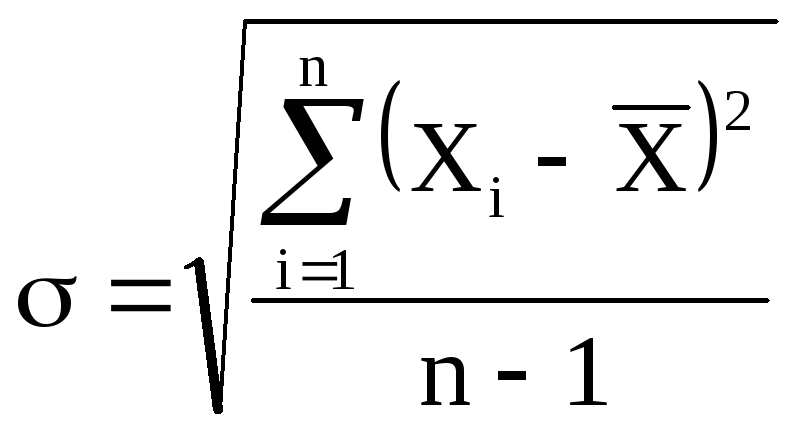
(5)
Величина
характеризует отклонение отдельного
единичного измерения от истинного
значения.
Если мы вычислили
по n
измерениям среднее значение
![]()
по формуле (2), то это значение будет
более точным, то есть будет меньше
отличаться от истинного, чем каждое
отдельное измерение. Средняя квадратичная
ошибка среднего значения
![]()
равна
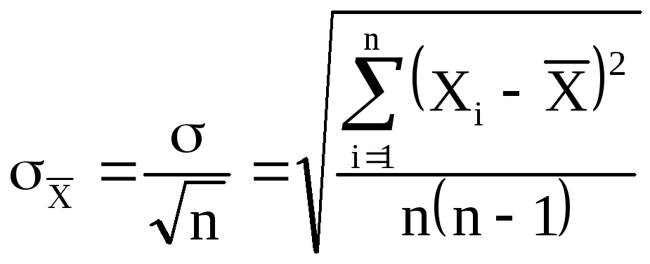
(6)
где — среднеквадратичная
ошибка каждого отдельного измерения,
n
– число
измерений.
Таким образом,
увеличивая число опытов, можно уменьшить
случайную ошибку в величине среднего
значения.
В настоящее время
результаты научных и технических
измерений принято представлять в виде
![]()
(7)
Как показывает
теория, при такой записи мы знаем
надежность полученного результата, а
именно, что истинная величина Х с
вероятностью 68% отличается от
![]()
не более, чем на
![]() .
.
При использовании
же средней арифметической (абсолютной)
ошибки (формула 2) о надежности результата
ничего сказать нельзя. Некоторое
представление о точности проведенных
измерений в этом случае дает относительная
ошибка (формула 4).
При выполнении
лабораторных работ студенты могут
использовать как среднюю абсолютную
ошибку, так и среднюю квадратичную.
Какую из них применять указывается
непосредственно в каждой конкретной
работе (или указывается преподавателем).
Обычно если число
измерений не превышает 3 – 5, то
можно использовать среднюю абсолютную
ошибку. Если число измерений порядка
10 и более, то следует использовать более
корректную оценку с
помощью средней квадратичной ошибки
среднего (формулы 5 и 6).
Учет систематических ошибок.
Увеличением числа
измерений можно уменьшить только
случайные ошибки опыта, но не
систематические.
Максимальное
значение систематической ошибки обычно
указывается на приборе или в его паспорте.
Для измерений с помощью обычной
металлической линейки систематическая
ошибка составляет не менее 0,5 мм; для
измерений штангенциркулем –
0,1 – 0,05 мм;
микрометром – 0,01 мм.
Часто в качестве
систематической ошибки берется половина
цены деления прибора.
На шкалах
электроизмерительных приборов указывается
класс точности. Зная класс точности К,
можно вычислить систематическую ошибку
прибора ∆Х по формуле
![]()
где К – класс
точности прибора, Хпр – предельное
значение величины, которое может быть
измерено по шкале прибора.
Так, амперметр
класса 0,5 со шкалой до 5А измеряет ток с
ошибкой не более
![]()
Среднее значение
полной погрешности складывается из
случайной и систематической
погрешностей.
![]()
Ответ с учетом
систематических и случайных ошибок
записывается в виде
![]()
Погрешности косвенных измерений
В физических
экспериментах чаще бывает так, что
искомая физическая величина сама на
опыте измерена быть не может, а является
функцией других величин, измеряемых
непосредственно. Например, чтобы
определить объём цилиндра, надо измерить
диаметр D и высоту h, а затем вычислить
объем по формуле
![]()
Величины D и h будут измерены с
некоторой ошибкой. Следовательно,
вычисленная величина
V
получится также с некоторой ошибкой.
Надо уметь выражать погрешность
вычисленной величины через погрешности
измеренных величин.
Как и при прямых
измерениях можно вычислять среднюю
абсолютную (среднюю арифметическую)
ошибку или среднюю квадратичную ошибку.
Общие правила
вычисления ошибок для обоих случаев
выводятся с помощью дифференциального
исчисления.
Пусть искомая
величина φ является функцией нескольких
переменных Х,
У, Z…
φ(Х,
У, Z…).
Путем прямых
измерений мы можем найти величины
![]() ,
,
а также оценить их средние абсолютные
ошибки
![]() …
…
или средние квадратичные ошибки Х,
У,
Z…
Тогда средняя
арифметическая погрешность
вычисляется по формуле
![]()
где
![]() — частные
— частные
производные от φ по
Х, У, Z. Они
вычисляются для средних значений
![]() …
…
Средняя квадратичная
погрешность вычисляется по формуле
![]()
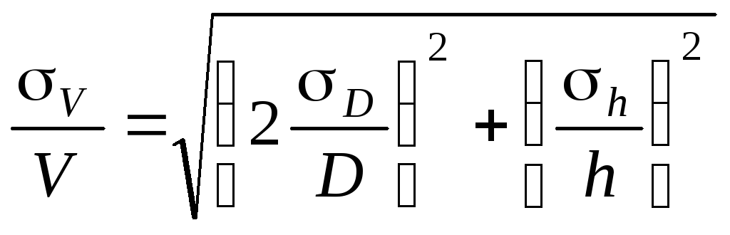
Пример.
Выведем формулы погрешности для
вычисления объёма цилиндра.
а) Средняя
арифметическая погрешность.
Величины
D и h
измеряются соответственно с ошибкой
D
и h.
Погрешность
величины объёма будет равна
![]()
б) Средняя
квадратичная погрешность.
Величины
D и h
измеряются соответственно с ошибкой
D, h.
Погрешность
величины объёма будет равна
![]()
Если формула
представляет выражение удобное для
логарифмирования (то есть произведение,
дробь, степень), то удобнее вначале
вычислять относительную погрешность.
Для этого (в случае средней арифметической
погрешности) надо проделать следующее.
1. Прологарифмировать
выражение.
2. Продифференцировать
его.
3. Объединить
все члены с одинаковым дифференциалом
и вынести его за скобки.
4. Взять выражение
перед различными дифференциалами по
модулю.
5. Заменить
значки дифференциалов d
на значки абсолютной погрешности .
В итоге получится
формула для относительной погрешности
![]()
Затем,
зная ,
можно вычислить абсолютную погрешность
=
Пример.
![]()
![]()
![]()
![]()
Аналогично можно
записать относительную среднюю
квадратичную погрешность
Правила
представления результатов измерения
следующие:
-
погрешность должна
округляться до одной значащей цифры:
правильно = 0,04,
неправильно —
= 0,0382;
-
последняя значащая
цифра результата должна быть того же
порядка величины, что и погрешность:
правильно
= 9,830,03,
неправильно —
= 9,8260,03;
-
если результат
имеет очень большую или очень малую
величину, необходимо использовать
показательную форму записи — одну и ту
же для результата и его погрешности,
причем запятая десятичной дроби должна
следовать за первой значащей цифрой
результата:
правильно —
= (5,270,03)10-5,
неправильно —
= 0,00005270,0000003,
= 5,2710-50,0000003,
=
= 0,0000527310-7,
= (5273)10-7,
= (0,5270,003)
10-4.
-
Если результат
имеет размерность, ее необходимо
указать:
правильно – g=(9,820,02)
м/c2,
неправильно – g=(9,820,02).
Соседние файлы в папке Отчеты_Погрешность
- #
- #
- #
- #
- #
Среднеквадратичная ошибка (Mean Squared Error) – Среднее арифметическое (Mean) квадратов разностей между предсказанными и реальными значениями Модели (Model) Машинного обучения (ML):

Рассчитывается с помощью формулы, которая будет пояснена в примере ниже:
$$MSE = frac{1}{n} × sum_{i=1}^n (y_i — widetilde{y}_i)^2$$
$$MSEspace{}{–}space{Среднеквадратическая}space{ошибка,}$$
$$nspace{}{–}space{количество}space{наблюдений,}$$
$$y_ispace{}{–}space{фактическая}space{координата}space{наблюдения,}$$
$$widetilde{y}_ispace{}{–}space{предсказанная}space{координата}space{наблюдения,}$$
MSE практически никогда не равен нулю, и происходит это из-за элемента случайности в данных или неучитывания Оценочной функцией (Estimator) всех факторов, которые могли бы улучшить предсказательную способность.
Пример. Исследуем линейную регрессию, изображенную на графике выше, и установим величину среднеквадратической Ошибки (Error). Фактические координаты точек-Наблюдений (Observation) выглядят следующим образом:

Мы имеем дело с Линейной регрессией (Linear Regression), потому уравнение, предсказывающее положение записей, можно представить с помощью формулы:
$$y = M * x + b$$
$$yspace{–}space{значение}space{координаты}space{оси}space{y,}$$
$$Mspace{–}space{уклон}space{прямой}$$
$$xspace{–}space{значение}space{координаты}space{оси}space{x,}$$
$$bspace{–}space{смещение}space{прямой}space{относительно}space{начала}space{координат}$$
Параметры M и b уравнения нам, к счастью, известны в данном обучающем примере, и потому уравнение выглядит следующим образом:
$$y = 0,5252 * x + 17,306$$
Зная координаты реальных записей и уравнение линейной регрессии, мы можем восстановить полные координаты предсказанных наблюдений, обозначенных серыми точками на графике выше. Простой подстановкой значения координаты x в уравнение мы рассчитаем значение координаты ỹ:

Рассчитаем квадрат разницы между Y и Ỹ:

Сумма таких квадратов равна 4 445. Осталось только разделить это число на количество наблюдений (9):
$$MSE = frac{1}{9} × 4445 = 493$$
Само по себе число в такой ситуации становится показательным, когда Дата-сайентист (Data Scientist) предпринимает попытки улучшить предсказательную способность модели и сравнивает MSE каждой итерации, выбирая такое уравнение, что сгенерирует наименьшую погрешность в предсказаниях.
MSE и Scikit-learn
Среднеквадратическую ошибку можно вычислить с помощью SkLearn. Для начала импортируем функцию:
import sklearn
from sklearn.metrics import mean_squared_error
Инициализируем крошечные списки, содержащие реальные и предсказанные координаты y:
y_true = [5, 41, 70, 77, 134, 68, 138, 101, 131]
y_pred = [23, 35, 55, 90, 93, 103, 118, 121, 129]
Инициируем функцию mean_squared_error(), которая рассчитает MSE тем же способом, что и формула выше:
mean_squared_error(y_true, y_pred)
Интересно, что конечный результат на 3 отличается от расчетов с помощью Apple Numbers:
496.0Ноутбук, не требующий дополнительной настройки на момент написания статьи, можно скачать здесь.
Автор оригинальной статьи: @mmoshikoo
Фото: @tobyelliott
Среднее квадратичное отклонение двух, трех, четырех и более чисел. Оно же стандартное отклонение, среднеквадратическое отклонение, среднеквадратичное отклонение, средняя квадратическая, стандартный разброс — показатель рассеивания значений случайной величины относительно её математического ожидания в теории вероятностей и статистике.
Как правило перечисленные термины равны квадратному корню дисперсии.
×
Для установки калькулятора на iPhone — просто добавьте страницу
«На главный экран»

Для установки калькулятора на Android — просто добавьте страницу
«На главный экран»

Смотрите также
![]()
Загрузить PDF
![]()
Загрузить PDF
После сбора данных их нужно проанализировать. Обычно нужно найти среднее значение, квадратичное отклонение и погрешность. Мы расскажем вам, как это сделать.
-

1
Запишите числовые значения, которые вы собираетесь анализировать. Мы проанализируем случайно подобранные числовые значения в качестве примера.
- Например, 5 школьникам был предложен письменный тест. Их результаты (в баллах по 100 бальной системе): 12, 55, 74, 79 и 90 баллов.
Реклама
-

1
Для того чтобы посчитать среднее значение, нужно сложить все имеющиеся числовые значения и разделить получившееся число на их количество.
- Среднее значение (μ) = Σ/N, где Σ сумма всех числовых значений, а N количество значений.
- То есть, в нашем случае μ равно (12+55+74+79+90)/5 = 62.
-

1
Мы будем считать среднее отклонение. Среднее отклонение = σ = квадратный корень из [(Σ((X-μ)^2))/(N)].
- Для вышеуказанного примера это квадратный корень из [((12-62)^2 + (55-62)^2 + (74-62)^2 + (79-62)^2 + (90-62)^2)/(5)] = 27,4. (Обратите внимание, что если это выборочное среднеквадратическое отклонение, то делить нужно на N-1, где N количество значений.)
Реклама
-

1
Считаем среднюю погрешность (среднего значения). Это оценка того, насколько сильно округляется общее среднее значение. Чем больше числовых значений, тем меньше средняя погрешность, тем точнее среднее значение. Для расчета погрешности надо разделить среднее отклонение на корень квадратный от N. Стандартная погрешность = σ/кв.корень(n).
- Если в нашем примере 5 школьников, а всего в классе 50 школьников, и среднее отклонение, посчитанное для 50 школьников равно 17 (σ = 21), средняя погрешность = 17/кв. корень(5) = 7.6.
Советы
- Расчеты среднего значения, среднего отклонения и погрешности годятся для анализа равномерно распределенных данных. Среднее отклонение математического среднего значения распределения относится приблизительно к 68% данных, 2 средних отклонения – к 95% данных, а 3 – к 99.7% данных. Стандартная погрешность же уменьшается при увеличении количества значений.
- Простой в использовании калькулятор для расчета среднего отклонения.
Реклама
Предупреждения
- Считайте дважды. Все делают ошибки.
Реклама
Об этой статье
Эту страницу просматривали 65 201 раз.
Была ли эта статья полезной?
В данной статье я расскажу о том, как найти среднеквадратическое отклонение. Этот материал крайне важен для полноценного понимания математики, поэтому репетитор по математике должен посвятить его изучению отдельный урок или даже несколько. В этой статье вы найдёте ссылку на подробный и понятный видеоурок, в котором рассказано о том, что такое среднеквадратическое отклонение и как его найти.
Среднеквадратическое отклонение дает возможность оценить разброс значений, полученных в результате измерения какого-то параметра. Обозначается символом  (греческая буква «сигма»).
Формула для расчета довольно проста. Чтобы найти среднеквадратическое отклонение, нужно взять квадратный корень из дисперсии. Так что теперь вы должны спросить: “А что же такое дисперсия?”
Что такое дисперсия
Определение дисперсии звучит так. Дисперсия — это среднее арифметическое от квадратов отклонений значений от среднего.
Чтобы найти дисперсию последовательно проведите следующие вычисления:
- Определите среднее (простое среднее арифметическое ряда значений).
- Затем от каждого из значений отнимите среднее и возведите полученную разность в квадрат (получили квадрат разности).
- Следующим шагом будет вычисление среднего арифметического полученных квадратов разностей (Почему именно квадратов вы сможете узнать ниже).
Рассмотрим на примере. Допустим, вы с друзьями решили измерить рост ваших собак (в миллиметрах). В результате измерений вы получили следующие данные измерений роста (в холке): 600 мм, 470 мм, 170 мм, 430 мм и 300 мм.
| Порода собаки | Рост в миллиметрах |
| Ротвейлер | 600 |
| Бульдог | 470 |
| Такса | 170 |
| Пудель | 430 |
| Мопс | 300 |
Вычислим среднее значение, дисперсию и среднеквадратическое отклонение.
Сперва найдём среднее значение. Как вы уже знаете, для этого нужно сложить все измеренные значения и поделить на количество измерений. Ход вычислений:
Среднее  мм.
мм.
Итак, среднее (среднеарифметическое) составляет 394 мм.
Теперь нужно определить отклонение роста каждой из собак от среднего:
![[ begin{array}{l} 1: 600-394 = 206 2: 470-394 = 76 3: 170-394 = -224 4: 430-394 = 36 5: 300-394 = -94 end{array} ]](https://yourtutor.info/wp-content/ql-cache/quicklatex.com-3916a3ccd97d909589dfe1dabb970af0_l3.png "Rendered by QuickLaTeX.com")
Наконец, чтобы вычислить дисперсию, каждую из полученных разностей возводим в квадрат, а затем находим среднее арифметическое от полученных результатов:
Дисперсия  мм2.
мм2.
Таким образом, дисперсия составляет 21704 мм2.
Как найти среднеквадратическое отклонение
Так как же теперь вычислить среднеквадратическое отклонение, зная дисперсию? Как мы помним, взять из нее квадратный корень. То есть среднеквадратическое отклонение равно:
 мм (округлено до ближайшего целого значения в мм).
Применив данный метод, мы выяснили, что некоторые собаки (например, ротвейлеры) – очень большие собаки. Но есть и очень маленькие собаки (например, таксы, только говорить им этого не стоит).
Самое интересное, что среднеквадратическое отклонение несет в себе полезную информацию. Теперь мы можем показать, какие из полученных результатов измерения роста находятся в пределах интервала, который мы получим, если отложим от среднего (в обе стороны от него) среднеквадратическое отклонение.
То есть с помощью среднеквадратического отклонения мы получаем “стандартный” метод, который позволяет узнать, какое из значений является нормальным (среднестатистическим), а какое экстраординарно большим или, наоборот, малым.
Что такое стандартное отклонение
Но… все будет немного иначе, если мы будем анализировать выборку данных. В нашем примере мы рассматривали генеральную совокупность. То есть наши 5 собак были единственными в мире собаками, которые нас интересовали.
Но если данные являются выборкой (значениями, которые выбрали из большой генеральной совокупности), тогда вычисления нужно вести иначе.
Если есть  значений, то:
Все остальные расчеты производятся аналогично, в том числе и определение среднего.
Например, если наших пять собак – только выборка из генеральной совокупности собак (всех собак на планете), мы должны делить на 4, а не на 5, а именно:
Дисперсия выборки =  мм2.
мм2.
При этом стандартное отклонение по выборке равно  мм (округлено до ближайшего целого значения).
Можно сказать, что мы произвели некоторую “коррекцию” в случае, когда наши значения являются всего лишь небольшой выборкой.
Примечание. Почему именно квадраты разностей?
Но почему при вычислении дисперсии мы берём именно квадраты разностей? Допустим при измерении какого-то параметра, вы получили следующий набор значений: 4; 4; -4; -4. Если мы просто сложим абсолютные отклонения от среднего (разности) между собой … отрицательные значения взаимно уничтожатся с положительными:
 .
.
Получается, этот вариант бесполезен. Тогда, может, стоит попробовать абсолютные значения отклонений (то есть модули этих значений)?
 .
.
На первый взгляд получается неплохо (полученная величина, кстати, называется средним абсолютным отклонением), но не во всех случаях. Попробуем другой пример. Пусть в результате измерения получился следующий набор значений: 7; 1; -6; -2. Тогда среднее абсолютное отклонение равно:
 .
.
Вот это да! Снова получили результат 4, хотя разности имеют гораздо больший разброс.
А теперь посмотрим, что получится, если возвести разности в квадрат (и взять потом квадратный корень из их суммы).
Для первого примера получится:
 .
.
Для второго примера получится:
 .
.
Теперь – совсем другое дело! Среднеквадратическое отклонение получается тем большим, чем больший разброс имеют разности … к чему мы и стремились.
Фактически в данном методе использована та же идея, что и при вычислении расстояния между точками, только примененная иным способом.
И с математической точки зрения использование квадратов и квадратных корней дает больше пользы, чем мы могли бы получить на основании абсолютных значений отклонений, благодаря чему среднеквадратическое отклонение применимо и для других математических задач.
О том, как найти среднеквадратическое отклонение, вам рассказал репетитор по математике в Москве, Сергей Валерьевич
Из предыдущей статьи мы узнали о таких показателях, как размах вариации, межквартильный размах и среднее линейное отклонение. В этой статье изучим дисперсию, среднеквадратичное отклонение и коэффициент вариации.
Дисперсия
Дисперсия случайной величины – это один из основных показателей в статистике. Он отражает меру разброса данных вокруг средней арифметической.
Сейчас небольшой экскурс в теорию вероятностей, которая лежит в основе математической статистики. Как и матожидание, дисперсия является важной характеристикой случайной величины. Если матожидание отражает центр случайной величины, то дисперсия дает характеристику разброса данных вокруг центра.
Формула дисперсии в теории вероятностей имеет вид:
![]()
То есть дисперсия — это математическое ожидание отклонений от математического ожидания.
На практике при анализе выборок математическое ожидание, как правило, не известно. Поэтому вместо него используют оценку – среднее арифметическое. Расчет дисперсии производят по формуле:
![]()
где
s2 – выборочная дисперсия, рассчитанная по данным наблюдений,
X – отдельные значения,
X̅– среднее арифметическое по выборке.
Стоит отметить, что у такого расчета дисперсии есть недостаток – она получается смещенной, т.е. ее математическое ожидание не равно истинному значению дисперсии. Подробней об этом здесь. Однако при увеличении объема выборки она все-таки приближается к своему теоретическому аналогу, т.е. является асимптотически не смещенной.
Простыми словами дисперсия – это средний квадрат отклонений. То есть вначале рассчитывается среднее значение, затем берется разница между каждым исходным и средним значением, возводится в квадрат, складывается и затем делится на количество значений в данной совокупности. Разница между отдельным значением и средней отражает меру отклонения. В квадрат возводится для того, чтобы все отклонения стали исключительно положительными числами и чтобы избежать взаимоуничтожения положительных и отрицательных отклонений при их суммировании. Затем, имея квадраты отклонений, просто рассчитываем среднюю арифметическую. Средний – квадрат – отклонений. Отклонения возводятся в квадрат, и считается средняя. Теперь вы знаете, как найти дисперсию.
Генеральную и выборочную дисперсии легко рассчитать в Excel. Есть специальные функции: ДИСП.Г и ДИСП.В соответственно.

В чистом виде дисперсия не используется. Это вспомогательный показатель, который нужен в других расчетах. Например, в проверке статистических гипотез или расчете коэффициентов корреляции. Отсюда неплохо бы знать математические свойства дисперсии.
Свойства дисперсии
Свойство 1. Дисперсия постоянной величины A равна 0 (нулю).
D(A) = 0
Свойство 2. Если случайную величину умножить на постоянную А, то дисперсия этой случайной величины увеличится в А2 раз. Другими словами, постоянный множитель можно вынести за знак дисперсии, возведя его в квадрат.
D(AX) = А2 D(X)
Свойство 3. Если к случайной величине добавить (или отнять) постоянную А, то дисперсия останется неизменной.
D(A + X) = D(X)
Свойство 4. Если случайные величины X и Y независимы, то дисперсия их суммы равна сумме их дисперсий.
D(X+Y) = D(X) + D(Y)
Свойство 5. Если случайные величины X и Y независимы, то дисперсия их разницы также равна сумме дисперсий.
D(X-Y) = D(X) + D(Y)
Среднеквадратичное (стандартное) отклонение
Если из дисперсии извлечь квадратный корень, получится среднеквадратичное (стандартное) отклонение (сокращенно СКО). Встречается название среднее квадратичное отклонение и сигма (от названия греческой буквы). Общая формула стандартного отклонения в математике следующая:
![]()
На практике формула стандартного отклонения следующая:
Как и с дисперсией, есть и немного другой вариант расчета. Но с ростом выборки разница исчезает.
Расчет cреднеквадратичного (стандартного) отклонения в Excel
Для расчета стандартного отклонения достаточно из дисперсии извлечь квадратный корень. Но в Excel есть и готовые функции: СТАНДОТКЛОН.Г и СТАНДОТКЛОН.В (по генеральной и выборочной совокупности соответственно).
 отклонение в Excel")
Среднеквадратичное отклонение имеет те же единицы измерения, что и анализируемый показатель, поэтому является сопоставимым с исходными данными.
Коэффициент вариации
Значение стандартного отклонения зависит от масштаба самих данных, что не позволяет сравнивать вариабельность разных выборках. Чтобы устранить влияние масштаба, необходимо рассчитать коэффициент вариации по формуле:
![]()
По нему можно сравнивать однородность явлений даже с разным масштабом данных. В статистике принято, что, если значение коэффициента вариации менее 33%, то совокупность считается однородной, если больше 33%, то – неоднородной. В реальности, если коэффициент вариации превышает 33%, то специально ничего делать по этому поводу не нужно. Это информация для общего представления. В общем коэффициент вариации используют для оценки относительного разброса данных в выборке.
Расчет коэффициента вариации в Excel
Расчет коэффициента вариации в Excel также производится делением стандартного отклонения на среднее арифметическое:
=СТАНДОТКЛОН.В()/СРЗНАЧ()
Коэффициент вариации обычно выражается в процентах, поэтому ячейке с формулой можно присвоить процентный формат:

Коэффициент осцилляции
Еще один показатель разброса данных на сегодня – коэффициент осцилляции. Это соотношение размаха вариации (разницы между максимальным и минимальным значением) к средней. Готовой формулы Excel нет, поэтому придется скомпоновать три функции: МАКС, МИН, СРЗНАЧ.

Коэффициент осцилляции показывает степень размаха вариации относительно средней, что также можно использовать для сравнения различных наборов данных.
Таким образом, в статистическом анализе существует система показателей, отражающих разброс или однородность данных.
Ниже видео о том, как посчитать коэффициент вариации, дисперсию, стандартное (среднеквадратичное) отклонение и другие показатели вариации в Excel.
Поделиться в социальных сетях:
17 авг. 2022 г.
читать 3 мин
В статистике регрессионный анализ — это метод, который мы используем для понимания взаимосвязи между переменной-предиктором x и переменной отклика y.
Когда мы проводим регрессионный анализ, мы получаем модель, которая сообщает нам прогнозируемое значение для переменной ответа на основе значения переменной-предиктора.
Один из способов оценить, насколько «хорошо» наша модель соответствует заданному набору данных, — это вычислить среднеквадратичную ошибку , которая представляет собой показатель, который говорит нам, насколько в среднем наши прогнозируемые значения отличаются от наших наблюдаемых значений.
Формула для нахождения среднеквадратичной ошибки, чаще называемая RMSE , выглядит следующим образом:
СКО = √[ Σ(P i – O i ) 2 / n ]
куда:
- Σ — причудливый символ, означающий «сумма».
- P i — прогнозируемое значение для i -го наблюдения в наборе данных.
- O i — наблюдаемое значение для i -го наблюдения в наборе данных.
- n — размер выборки
Технические примечания:
- Среднеквадратичную ошибку можно рассчитать для любого типа модели, которая дает прогнозные значения, которые затем можно сравнить с наблюдаемыми значениями набора данных.
- Среднеквадратичную ошибку также иногда называют среднеквадратичным отклонением, которое часто обозначается аббревиатурой RMSD.
Далее рассмотрим пример расчета среднеквадратичной ошибки в Excel.
Как рассчитать среднеквадратичную ошибку в Excel
В Excel нет встроенной функции для расчета RMSE, но мы можем довольно легко вычислить его с помощью одной формулы. Мы покажем, как рассчитать RMSE для двух разных сценариев.
Сценарий 1
В одном сценарии у вас может быть один столбец, содержащий предсказанные значения вашей модели, и другой столбец, содержащий наблюдаемые значения. На изображении ниже показан пример такого сценария:
Если это так, то вы можете рассчитать RMSE, введя следующую формулу в любую ячейку, а затем нажав CTRL+SHIFT+ENTER:
=КОРЕНЬ(СУММСК(A2:A21-B2:B21) / СЧЕТЧ(A2:A21))
Это говорит нам о том, что среднеквадратическая ошибка равна 2,6646 .
Формула может показаться немного сложной, но она имеет смысл, если ее разобрать:
= КОРЕНЬ( СУММСК(A2:A21-B2:B21) / СЧЕТЧ(A2:A21) )
- Во-первых, мы вычисляем сумму квадратов разностей между прогнозируемыми и наблюдаемыми значениями, используя функцию СУММСК() .
- Затем мы делим на размер выборки набора данных, используя COUNTA() , который подсчитывает количество непустых ячеек в диапазоне.
- Наконец, мы извлекаем квадратный корень из всего вычисления, используя функцию SQRT() .
Сценарий 2
В другом сценарии вы, возможно, уже вычислили разницу между прогнозируемыми и наблюдаемыми значениями. В этом случае у вас будет только один столбец, отображающий различия.
На изображении ниже показан пример этого сценария. Прогнозируемые значения отображаются в столбце A, наблюдаемые значения — в столбце B, а разница между прогнозируемыми и наблюдаемыми значениями — в столбце D:
Если это так, то вы можете рассчитать RMSE, введя следующую формулу в любую ячейку, а затем нажав CTRL+SHIFT+ENTER:
=КОРЕНЬ(СУММСК(D2:D21) / СЧЕТЧ(D2:D21))
Это говорит нам о том, что среднеквадратическая ошибка равна 2,6646 , что соответствует результату, полученному в первом сценарии. Это подтверждает, что эти два подхода к расчету RMSE эквивалентны.
Формула, которую мы использовали в этом сценарии, лишь немного отличается от той, что мы использовали в предыдущем сценарии:
= КОРЕНЬ (СУММСК(D2 :D21) / СЧЕТЧ(D2:D21) )
- Поскольку мы уже рассчитали разницу между предсказанными и наблюдаемыми значениями в столбце D, мы можем вычислить сумму квадратов разностей с помощью функции СУММСК().только со значениями в столбце D.
- Затем мы делим на размер выборки набора данных, используя COUNTA() , который подсчитывает количество непустых ячеек в диапазоне.
- Наконец, мы извлекаем квадратный корень из всего вычисления, используя функцию SQRT() .
Как интерпретировать среднеквадратичную ошибку
Как упоминалось ранее, RMSE — это полезный способ увидеть, насколько хорошо регрессионная модель (или любая модель, которая выдает прогнозируемые значения) способна «соответствовать» набору данных.
Чем больше RMSE, тем больше разница между прогнозируемыми и наблюдаемыми значениями, а это означает, что модель регрессии хуже соответствует данным. И наоборот, чем меньше RMSE, тем лучше модель соответствует данным.
Может быть особенно полезно сравнить RMSE двух разных моделей друг с другом, чтобы увидеть, какая модель лучше соответствует данным.
Для получения дополнительных руководств по Excel обязательно ознакомьтесь с нашей страницей руководств по Excel , на которой перечислены все учебные пособия Excel по статистике.
Средняя квадратичная ошибка.
При ответственных
измерениях, когда необходимо знать
надежность полученных результатов,
используется средняя квадратичная
ошибка (или
стандартное отклонение), которая
определяется формулой
(5)
Величина
характеризует отклонение отдельного
единичного измерения от истинного
значения.
Если мы вычислили
по n
измерениям среднее значение
![]()
по формуле (2), то это значение будет
более точным, то есть будет меньше
отличаться от истинного, чем каждое
отдельное измерение. Средняя квадратичная
ошибка среднего значения
![]()
равна
(6)
где — среднеквадратичная
ошибка каждого отдельного измерения,
n
– число
измерений.
Таким образом,
увеличивая число опытов, можно уменьшить
случайную ошибку в величине среднего
значения.
В настоящее время
результаты научных и технических
измерений принято представлять в виде
![]()
(7)
Как показывает
теория, при такой записи мы знаем
надежность полученного результата, а
именно, что истинная величина Х с
вероятностью 68% отличается от
![]()
не более, чем на
![]() .
.
При использовании
же средней арифметической (абсолютной)
ошибки (формула 2) о надежности результата
ничего сказать нельзя. Некоторое
представление о точности проведенных
измерений в этом случае дает относительная
ошибка (формула 4).
При выполнении
лабораторных работ студенты могут
использовать как среднюю абсолютную
ошибку, так и среднюю квадратичную.
Какую из них применять указывается
непосредственно в каждой конкретной
работе (или указывается преподавателем).
Обычно если число
измерений не превышает 3 – 5, то
можно использовать среднюю абсолютную
ошибку. Если число измерений порядка
10 и более, то следует использовать более
корректную оценку с
помощью средней квадратичной ошибки
среднего (формулы 5 и 6).
Учет систематических ошибок.
Увеличением числа
измерений можно уменьшить только
случайные ошибки опыта, но не
систематические.
Максимальное
значение систематической ошибки обычно
указывается на приборе или в его паспорте.
Для измерений с помощью обычной
металлической линейки систематическая
ошибка составляет не менее 0,5 мм; для
измерений штангенциркулем –
0,1 – 0,05 мм;
микрометром – 0,01 мм.
Часто в качестве
систематической ошибки берется половина
цены деления прибора.
На шкалах
электроизмерительных приборов указывается
класс точности. Зная класс точности К,
можно вычислить систематическую ошибку
прибора ∆Х по формуле
![]()
где К – класс
точности прибора, Хпр – предельное
значение величины, которое может быть
измерено по шкале прибора.
Так, амперметр
класса 0,5 со шкалой до 5А измеряет ток с
ошибкой не более
![]()
Среднее значение
полной погрешности складывается из
случайной и систематической
погрешностей.
![]()
Ответ с учетом
систематических и случайных ошибок
записывается в виде
![]()
Погрешности косвенных измерений
В физических
экспериментах чаще бывает так, что
искомая физическая величина сама на
опыте измерена быть не может, а является
функцией других величин, измеряемых
непосредственно. Например, чтобы
определить объём цилиндра, надо измерить
диаметр D и высоту h, а затем вычислить
объем по формуле
![]()
Величины D и h будут измерены с
некоторой ошибкой. Следовательно,
вычисленная величина
V
получится также с некоторой ошибкой.
Надо уметь выражать погрешность
вычисленной величины через погрешности
измеренных величин.
Как и при прямых
измерениях можно вычислять среднюю
абсолютную (среднюю арифметическую)
ошибку или среднюю квадратичную ошибку.
Общие правила
вычисления ошибок для обоих случаев
выводятся с помощью дифференциального
исчисления.
Пусть искомая
величина φ является функцией нескольких
переменных Х,
У, Z…
φ(Х,
У, Z…).
Путем прямых
измерений мы можем найти величины
![]() ,
,
а также оценить их средние абсолютные
ошибки
![]() …
…
или средние квадратичные ошибки Х,
У,
Z…
Тогда средняя
арифметическая погрешность
вычисляется по формуле
![]()
где
![]() — частные
— частные
производные от φ по
Х, У, Z. Они
вычисляются для средних значений
![]() …
…
Средняя квадратичная
погрешность вычисляется по формуле
![]()
Пример.
Выведем формулы погрешности для
вычисления объёма цилиндра.
а) Средняя
арифметическая погрешность.
Величины
D и h
измеряются соответственно с ошибкой
D
и h.
Погрешность
величины объёма будет равна
![]()
б) Средняя
квадратичная погрешность.
Величины
D и h
измеряются соответственно с ошибкой
D, h.
Погрешность
величины объёма будет равна
![]()
Если формула
представляет выражение удобное для
логарифмирования (то есть произведение,
дробь, степень), то удобнее вначале
вычислять относительную погрешность.
Для этого (в случае средней арифметической
погрешности) надо проделать следующее.
1. Прологарифмировать
выражение.
2. Продифференцировать
его.
3. Объединить
все члены с одинаковым дифференциалом
и вынести его за скобки.
4. Взять выражение
перед различными дифференциалами по
модулю.
5. Заменить
значки дифференциалов d
на значки абсолютной погрешности .
В итоге получится
формула для относительной погрешности
![]()
Затем,
зная ,
можно вычислить абсолютную погрешность
=
Пример.
![]()
![]()
![]()
![]()
Аналогично можно
записать относительную среднюю
квадратичную погрешность
Правила
представления результатов измерения
следующие:
-
погрешность должна
округляться до одной значащей цифры:
правильно = 0,04,
неправильно —
= 0,0382;
-
последняя значащая
цифра результата должна быть того же
порядка величины, что и погрешность:
правильно
= 9,830,03,
неправильно —
= 9,8260,03;
-
если результат
имеет очень большую или очень малую
величину, необходимо использовать
показательную форму записи — одну и ту
же для результата и его погрешности,
причем запятая десятичной дроби должна
следовать за первой значащей цифрой
результата:
правильно —
= (5,270,03)10-5,
неправильно —
= 0,00005270,0000003,
= 5,2710-50,0000003,
=
= 0,0000527310-7,
= (5273)10-7,
= (0,5270,003)
10-4.
-
Если результат
имеет размерность, ее необходимо
указать:
правильно – g=(9,820,02)
м/c2,
неправильно – g=(9,820,02).
Соседние файлы в папке Отчеты_Погрешность
- #
- #
- #
- #
- #
Среднеквадратичная ошибка (Mean Squared Error) – Среднее арифметическое (Mean) квадратов разностей между предсказанными и реальными значениями Модели (Model) Машинного обучения (ML):
Рассчитывается с помощью формулы, которая будет пояснена в примере ниже:
$$MSE = frac{1}{n} × sum_{i=1}^n (y_i — widetilde{y}_i)^2$$
$$MSEspace{}{–}space{Среднеквадратическая}space{ошибка,}$$
$$nspace{}{–}space{количество}space{наблюдений,}$$
$$y_ispace{}{–}space{фактическая}space{координата}space{наблюдения,}$$
$$widetilde{y}_ispace{}{–}space{предсказанная}space{координата}space{наблюдения,}$$
MSE практически никогда не равен нулю, и происходит это из-за элемента случайности в данных или неучитывания Оценочной функцией (Estimator) всех факторов, которые могли бы улучшить предсказательную способность.
Пример. Исследуем линейную регрессию, изображенную на графике выше, и установим величину среднеквадратической Ошибки (Error). Фактические координаты точек-Наблюдений (Observation) выглядят следующим образом:
Мы имеем дело с Линейной регрессией (Linear Regression), потому уравнение, предсказывающее положение записей, можно представить с помощью формулы:
$$y = M * x + b$$
$$yspace{–}space{значение}space{координаты}space{оси}space{y,}$$
$$Mspace{–}space{уклон}space{прямой}$$
$$xspace{–}space{значение}space{координаты}space{оси}space{x,}$$
$$bspace{–}space{смещение}space{прямой}space{относительно}space{начала}space{координат}$$
Параметры M и b уравнения нам, к счастью, известны в данном обучающем примере, и потому уравнение выглядит следующим образом:
$$y = 0,5252 * x + 17,306$$
Зная координаты реальных записей и уравнение линейной регрессии, мы можем восстановить полные координаты предсказанных наблюдений, обозначенных серыми точками на графике выше. Простой подстановкой значения координаты x в уравнение мы рассчитаем значение координаты ỹ:
Рассчитаем квадрат разницы между Y и Ỹ:
Сумма таких квадратов равна 4 445. Осталось только разделить это число на количество наблюдений (9):
$$MSE = frac{1}{9} × 4445 = 493$$
Само по себе число в такой ситуации становится показательным, когда Дата-сайентист (Data Scientist) предпринимает попытки улучшить предсказательную способность модели и сравнивает MSE каждой итерации, выбирая такое уравнение, что сгенерирует наименьшую погрешность в предсказаниях.
MSE и Scikit-learn
Среднеквадратическую ошибку можно вычислить с помощью SkLearn. Для начала импортируем функцию:
import sklearn
from sklearn.metrics import mean_squared_error
Инициализируем крошечные списки, содержащие реальные и предсказанные координаты y:
y_true = [5, 41, 70, 77, 134, 68, 138, 101, 131]
y_pred = [23, 35, 55, 90, 93, 103, 118, 121, 129]
Инициируем функцию mean_squared_error(), которая рассчитает MSE тем же способом, что и формула выше:
mean_squared_error(y_true, y_pred)
Интересно, что конечный результат на 3 отличается от расчетов с помощью Apple Numbers:
496.0Ноутбук, не требующий дополнительной настройки на момент написания статьи, можно скачать здесь.
Автор оригинальной статьи: @mmoshikoo
Фото: @tobyelliott