Empirical Bayes and hierarchical models
K. Friston, W. Penny, in Statistical Parametric Mapping, 2007
The conditional density
Given an estimate of the error covariance of the augmented form Cε and implicitly the priors it entails, one can compute the conditional mean and covariance at each level where the conditional means for each level obtain recursively from:
22.19ηθ|y=E(θ|y)=[ηɛ|y(2)⋮ηɛ|y(n)ηθ|y(n)]ηθ|y(i−1)=E(θ(i−1)y)=X(i)ηθ|y(i)+ηɛ|y(i)
These conditional expectations represent a better characterization of the model parameters than the equivalent ML estimates because they are constrained by higher levels (see summary). However, the conditional mean and ML estimators are the same at the last level. This convergence of classical and Bayesian inference rests on adopting an empirical Bayesian approach and establishes a close connection between classical random effect analyses and hierarchical Bayesian models. The two approaches diverge if we consider that the real power of Bayesian inference lies in coping with incomplete data or unbalanced designs and inferring on the parameters of lower levels. These are the issues considered in the next section.
Read full chapter
URL:
https://www.sciencedirect.com/science/article/pii/B978012372560850022X
Volume 2
P.D. Wentzell, in Comprehensive Chemometrics, 2009
2.25.3.3.2 Theoretical modeling
An alternative approach to estimating the error covariance matrix by replication is to use fundamental knowledge about the measurement system to build the error covariance matrix. The specific strategy used can range from imposing intuitive knowledge derived from a familiarity with the system under study to more rigorous modeling of the overall measurement system. In the first category, for example, one may have observed that the measurements follow a proportional error structure, or may simply not have as much confidence in one group of measurements compared to another. While MLPCA will only provide truly optimal models if the error structure provided is correct, a feature of the method is that the model will generally become better as information about the error structure is incrementally refined. Therefore, even partial or approximate knowledge of the nature of the noise can be beneficial. Moreover, absolute values for variances and covariances need not be provided since the maximum likelihood projection depends only on the relative values.
In terms of more rigorous modeling of the error structure, a considerable body of knowledge has been developed on the nature of signals from various types of instruments and their limiting sources of noise (e.g., shot noise, source flicker noise, detector noise).16 Such information could be used to develop more refined error information, but there are a couple of limitations to this approach. First, while the instruments may be fairly well characterized, the measurement systems as a whole may introduce some other dominant source of error. For example, assuming that fluorescence measurements are shot-noise limited may be accurate from a signal detection perspective, but the overall error may be dominated by cell positioning, preparation, or sampling errors. A second limitation of this approach is that most noise models have focused on variance and do not tackle the more difficult problem of covariance, which can be tied to specific design factors and signal processing methods.
One special case where theoretical modeling of covariance structure is straightforward is when digital filtering is used. This technique has already been employed in this chapter to generate correlated errors for simulated data. Under these circumstances, the error covariance matrix can be derived directly from the filter. To do this, it is most convenient to describe the filtering process in terms of a filter matrix, F, such that Dfilt = DorigFT, where Dfilt is the filtered data matrix and Dorig is the original data matrix. Typically, F is a band diagonal matrix of filter coefficients, although special considerations have to be made near the edges. Under these conditions, the error covariance matrix for the filtered data will be given by
(81)Σfilt=FΣorigFT
Of course, this still requires a knowledge of the error covariance matrix for the original data, Σorig, but if it can be assumed to be i.i.d. normal, the effect of digital filtering is easy to predict.
The advantages of the theoretical modeling approach are as follows: (1) it eliminates the need for performing replicate measurements; (2) there is no stochastic noise in the error covariance estimates; (3) it is likely to be able to be generalized to all of the measurements made on the same instrument; and (4) the anomalous projection of replicates onto the sample mean is avoided. Unfortunately, coming up with an accurate model on a purely theoretical basis is not likely to be realistic given all of the potential sources of variance and covariance in the noise. Normally, the best that can be hoped for under these circumstances is a model that is better than the assumption of i.i.d. errors. However, another approach is to combine replicate measurements with theoretical modeling, as described in the next section.
Read full chapter
URL:
https://www.sciencedirect.com/science/article/pii/B9780444527011000570
Selection of Manifest Variables*
Yutaka Kano, in Handbook of Latent Variable and Related Models, 2007
4.1 Model with correlated errors
Probably it was Bollen (1980) who first emphasized importance of introducing error covariances in researches using factor analysis. We shall reanalyze the data set in Section 3.1 to achieve a good fit not by removing manifest variables but by allowing error covariances. We analyzed it with the help of LM tests offered by EQS (Bentler, 2004). The path diagram of a final model is shown in Figure 4. Fit indices of the final model are χ2 = 250.375 (df = 83, n = 653), GFI = 0.950, CFI = 0.952, RMSEA = 0.056. Those statistics indicate a fairly good fit.

Fig. 4. The final model with error covariances.
Recall that SEFA suggests deletion of the variables X2, X9, X13 and X14. We see that SEFA chooses such variables to be removed that those error covariances are eliminated. As a result, the final model with 11 manifest variables is a factor analysis model with uncorrelated errors. This is an interpretation of how SEFA suggests manifest variables to be removed. This gives an answer to question (a). Note that there is some freedom in eliminating error covariances. For example, if either X8 or X9 is removed, the covariance between E8 and E9 can be eliminated. If the model in Figure 4 is true, the choice between X8 and X9 is completely arbitrary from the viewpoint of a model fit. The situation is slightly more complicated for the variables X11 to X14. It is possible to remove three of the four variables. Oka et al. (2002) dropped a total of five variables slightly different from ours by taking into account the meaning of the variables.
There are many cases where it is relevant to introduce error covariances, one of which is the case where there exist confounding third unmeasured variables that connect two or more manifest variables. A method factor is a typical example of confounding variables in studies of social sciences. While common factors cannot usually explain covariances between manifest variables caused by method factors, error covariances can explain them. Method factors are often discussed in the analysis of MTMM matrices (e.g., Campbell and Fiske, 1959; Campbell and O’Connell, 1967).
Green and Hershberger (2000) suggested several kinds of measurement models for longitudinal data. One of their models is a true score model with a moving average component of order one given in Figure 5 (left). The model is equivalent to a one-factor analysis model with errors correlated next to each other (Figure 5 (right)).

Fig. 5. A model with a moving average component of order one and its equivalent model.
A third one is nonlinearity. Suppose that the following nonlinear factor analysis model holds:
X1=μ1+λ11f+λ12f2+e1X2=μ2+λ21f+λ22f2+e2X3=μ3+λ31f+e3⋯Xp=μp+λp1f+ep
where the usual assumptions of a factor analysis model are made. Assuming that the distribution of f1 is symmetric about the origin, we have Cov(f, f2) = 0, and Cov(λ12f2 + e1, λ22f2 + e2) = λ12λ22 Var(f2) (≠ 0) results in an error covariance. When the effect of quadratic terms is not large and does not interest the researcher, one can approximate the effect of f by the linear terms, and the quadratic terms can be regarded as errors. See Lee and Zhu (2002) for general theory of nonlinear structural equation models.
What happens if there exist error covariances in the model and one fits a model without error covariances? A fit of the model will be poor. In addition, factor loadings and communality estimates can be biased. This problem will be discussed in the next section. Which model to employ becomes an issue: a model removing some manifest variables or a model introducing error covariances. We shall discuss this issue in the context of reliability analysis in the next section.
Read full chapter
URL:
https://www.sciencedirect.com/science/article/pii/B9780444520449500070
The General Linear Model
S.J. Kiebel, … C. Holmes, in Statistical Parametric Mapping, 2007
Estimation of the error covariance matrix
Assuming that the AR(1) + wn is an appropriate model for the fMRI error covariance matrix, we need to estimate three hyperparameters (see Appendix 8.1) at each voxel. The hyperparameterized model gives a covariance matrix at each voxel (Eqn. 8.45). In SPM, an additional assumption is made to estimate this matrix very efficiently, which is described in the following.
The error covariance matrix can be partitioned into two components. The first component is the correlation matrix and the second is the variance. The assumption made by SPM is that the correlation matrix is the same at all voxels of interest (see Chapter 10 for further details).
The variance is assumed to differ between voxels. In other words, SPM assumes that the pattern of serial correlations is the same over all interesting voxels, but its amplitude is different at each voxel. This assumption seems to be quite sensible, because the serial correlations over voxels within tissue types are usually very similar. The ensuing estimate of the serial correlations is extremely precise because one can pool information from the subset of voxels involved in the estimation. This means the correlation matrix at each voxel can be treated as a known and fixed quantity in subsequent inference.
The estimation of the error covariance matrix proceeds as follows. Let us start with the linear model for voxel k:
where Yk is an N × 1 observed time-series vector at voxel k, X is an N × L design matrix, βk is the parameter vector and ek is the error at voxel k. The error ɛk is normally distributed with ɛ˜N(0,σk2V) The critical difference, in relation to Eqn. 8.6, is the distribution of the error; where the identity matrix I is replaced by the correlation matrix V. Note that V does not depend on the voxel position k, i.e. as mentioned above we assume that the correlation matrix V is the same for all voxels k = 1, …, K. However, the variance σk2 is different for each voxel.
Since we assume that V is the same at each voxel, we can pool data from all voxels and then estimate V on this pooled data. The pooled data are given by summing the sampled covariance matrix of all interesting voxels k, i.e. Vϒ=1/KΣkϒkϒkT Note that the pooled VY is a mixture of two variance components; the experimentally induced variance and the error variance component:
The conventional way to estimate the components of the error covariance matrix Cov(ɛk) = σk2 V is to use restricted maximum likelihood (ReML) (Harville, 1997; Friston et al., 2002). ReML returns an unbiased estimator of the covariance components, while accounting for uncertainty about the parameter estimates. ReML can work with precision or covariance components; in our case we need to estimate a mixture of covariance components. The concept of covariance components is a very general concept that can be used to model all kinds of non-sphericity (see Chapter 10). The model described in Appendix 8.1 (Eqn. 8.44) is non-linear in the hyperparameters, so ReML cannot be used directly. But if we use a linear approximation:
where Ql are N × N components and the λl are the hyperparameters, ReML can be applied. We want to specifyQl such that they form an appropriate model for serial correlations in fMRI data. The default model in SPM is to use two components Q1 and Q2. These are Q1 = IN and:
8.38Q2ij={e−|i−j|:i≠j0:i=j
Figure 8.16 shows the shape of Q1 and Q2.

FIGURE 8.16. Graphical illustration of the two covariance components, which are used for estimating serial correlations. Left: component Q1 that corresponds to a stationary white variance component; right: components Q2 that implements the AR(1) part with an autoregression coefficient of 1/e.
A voxel-wide estimate of V is then derived by re-scaling V such that V is a correlation matrix.
This method of estimating the covariance matrix at each voxel uses the two voxel-wide (global) hyperparameters λ1 and λ2. A third voxel-wise (local) hyperparameter (the variance Σ2) is estimated at each voxel using the usual estimator in a least squares mass-univariate scheme (Worsley and Friston, 1995):
where R is the residual forming matrix. This completes the estimation of the serial correlations at each voxel k. Before we can use these estimates to derive statistical tests, we will consider the highpass filter and the role it plays in modelling fMRI data.
Read full chapter
URL:
https://www.sciencedirect.com/science/article/pii/B9780123725608500085
Kalman Filters and Nonlinear Filters
Vytas B. Gylys, in Encyclopedia of Physical Science and Technology (Third Edition), 2003
IV.B Square Root Filtering
By far the greatest trouble spot in computer mechanization of the KF is the updating of state error covariance matrix P, that is, the computation of Pk∣k according to Eq. (18). As the estimation process progresses, the elements of Pk∣k typically continue to decrease in magnitude and so matrix Pk∣k keeps approaching the zero matrix, although theoretically it should forever remain positive definite, no matter how small in magnitude its elements become. Hence, unless special measures are taken, accumulation of roundoff error in the repetitive use of Eq. (18) may cause the computed Pk∣k to lose its positive definiteness. As suggested by the matrix inversion operation appearing on the right-hand side of Eq. (16) for computing the Kalman gain, this situation is aggravated if several components of the measurement vector are very accurate and consequently the positive definite measurement error covariance matrix R is ill conditioned, that is, if R has eigenvalues of both relatively very large and small magnitudes.
Let A be a nonnegative definite symmetric matrix; then there exists a matrix S such that A = SST. Matrix S is often called the square root of A. The Cholesky decomposition algorithm provides a method of constructing from A the matrix S so that S is lower triangular; that is, all elements of S above the main diagonal are zero. Square root filtering is motivated by the observations that, if the state error covariance matrix P = SST, then (a) since SST is always nonnegative definite, matrix P expressed as SST cannot become negative definite, and (b) matrix S is generally less ill conditioned than matrix P.
Several versions of the square root filtering algorithm are known. The earliest form was developed by J. E. Potter in 1964 for applications in which the process noise is absent (i.e., covariance matrix Q is zero) and the measurements are sequentially processed as scalars. In 1967 J. F. Bellantoni and K. W. Dodge extended Potter’s results to vector-valued measurements. A. Andrews in 1968 and then S. F. Schmidt in 1970 published two alternative procedures for handling the process noise. In 1973 N. A. Carlson described a procedure that considerably improved the speed and decreased the memory requirements of square root filtering and in which, as in Potter’s algorithm, vector-valued measurements are processed sequentially as scalars. Finally, the so-called UDUT covariance factorization method is the most recent major milestone in numerical handling of KFs. This method, developed by G. J. Bierman and C. L. Thornton, represents the state error covariances before and after the measurement update step asPk|k−1=Uk|k−1Dk|k−1Uk|k−1TandPk|k=Uk|kDk|kUk|kT,with D being a diagonal matrix and U an upper triangular matrix with 1’s on its main diagonal. In this method, the square root of the covariance matrix, which now would correspond to UD1/2, is never computed explicitly, which avoids numerical computation of square roots. Like Carlson’s algorithm, the UDUT factorization method maintains the covariance matrix in factored form and so (like Carlson’s algorithm) is considerably more efficient in processor time and storage than the original Potter algorithm.
As a quick comparison of computational efficiency, the conventional Kalman method, the less efficient form of Carlson’s algorithm, and the UDUT factorization method are roughly equal: The processing of each time step (consisting of one time propagation and one measurement update) requires of the order of 16[9ns3 + 9ns2nm + 3ns2nw] adds and about the same number of multiplies, plus a relatively modest number of divides and square roots (square roots are required only in some, as in Potter’s or Carlson’s square root algorithms). Here, as before, ns is the length of the state vector, nm the length of the measurement vector, and nw the lenght of the process noise vector w. The faster version of Carlson’s algorithm is more efficient and requires only of the order of 16[5ns3 + 9ns2nm + 3ns2nw] adds and 16[5ns3 + 12ns2nm + 3ns2nw] multiplies, plus 2nsnm divides and nsnm square roots, at each time point. The stable (Joseph) form of the KF [as given by Eq. (18′)] fares more poorly: At each time step, it requires of the order of 16[18ns3 + 15ns2nm + 3ns2nw] adds and about the same number of multiplies.
As a summary, (a) a square root filter is a numerically stable form for performing the KF covariance–gain processing defined by Eqs. (15), (16), and (18); (b) the efficiency of its more recent versions roughly compares with that of these three equations; (c) the increased stability allows one to use relatively low-precision arithmetic in the KF gain–covariance processing, with a possible exception of some dot products.
Real-time implementation of a filter involves additional issues that are unimportant in the non-real-time environment. Besides the adequacy of functional performance, the most important of these issues is the requirement to produce timely responses to external stimuli. Thus, resorting to a parallel or concurrent processing may be the only way out. This usually implies the use of special hardware architectures such as parallel, vector pipelined, or systolic processors.
As one example, consider the use of a filter in the tracking of multiple objects in a hard real-time environment characterized by strict deadlines. In such a case one may want to maintain simultaneously many estimation processes, each handling a single object. Parallel processors may seem to be a suitable hardware architecture for this problem, but if separate estimation processes in such an application progress at different rates and at any time some of them require a great amount of special handling, then parallel architecture, such as a single-instruction multiple-data stream computer, may not be the best choice. As another example, consider a KF to be implemented as part of a navigation system on a small airborne computer (uniprocessor). Suppose that the navigation measurements come at a certain fixed rate. If the filtering process cannot keep up with the arrival rate of measurements and so not all of them can be utilized, the estimation performance may deteriorate. In this problem, if there is an upper bound on hardware resources, the only solution may be to decompose the estimation algorithm into concurrently executable processes. For instance, the time-propagation step (which, say, is to be executed at a relatively high rate) may constitute one process and the measurement-update step (which needs to be executed only at some lower rate, say, at the rate of measurement arrivals) may constitute another. Such a decomposition of an estimation algorithm into concurrent procedures often creates a surrogate algorithm that performs more poorly than the original algorithm.
The effects of the finite-length word computing is another issue that must be considered in filter implementation for real-time applications. The computer on which a filter is developed and validated through successive off-line simulations is often more powerful and uses higher-precision arithmetic and number representations than the ultimate real-time processor. Hence, one must in advance determine in advance what effect a shorter word length will have on performance.
Read full chapter
URL:
https://www.sciencedirect.com/science/article/pii/B0122274105003574
Bayesian model selection and averaging
W.D. Penny, … N. Trujillo-Barreto, in Statistical Parametric Mapping, 2007
Variance components
Bayesian estimation, as described in the previous section, assumed that we knew the prior covariance, Cp, and error covariance, Ce. This information is, however, rarely available. In Friston et al. (2002)) these covariances are expressed as:
where Qi and Qj are known as ‘covariance components’ and λi, λj are hyperparameters. Chapter 24 and Friston et al. (2002)) show how these hyperparameters can be estimated using parametric empirical Bayes (PEB). It is also possible to represent precision matrices, rather than covariance matrices, using a linear expansion as shown in Appendix 4.
Read full chapter
URL:
https://www.sciencedirect.com/science/article/pii/B9780123725608500358
Special Volume: Computational Methods for the Atmosphere and the Oceans
Jacques Blum, … I. Michael Navon, in Handbook of Numerical Analysis, 2009
7.13 Covariance localization
One aspect of ensemble assimilation methods is the requirement of accuracy for covariance matrices. Erroneous representation of error statistics affects the analysis-error covariance, which is propagated forward in time.
The covariance estimate from the ensemble is multiplied point by point with a correlation function that is 1.0 at the observation location and zero beyond some prespecified distance (correlation length).
Two approaches are used: one consists in a cut-off radius so that observations are not assimilated beyond a certain distance from the grid point (see Houtekamer and Mitchell [1998], Evensen [2003]). This may introduce spurious discontinuities.
The second approach is to use a correlation function that decreases monotonically with increasing distance. This results in the Kalman gain
(7.25)K=PbHT(HPbHT+R)−1,
being replaced by a modified gain
(7.26)K=(ρsоPb)HT(H(ρsоPb)HT+R)−1,
where the operation ρsо denotes a Schur product (an element-by-element multiplication) of a correlation matrix S with local support with the covariance model generated by the ensemble. The Schur product of matrices A and B is a matrix C of the same dimension, where cij= aijbij. When covariance localization is applied to smaller ensembles, it may result in more accurate analyses than would be obtained from larger ensembles without localization Houtekamer and Mitchell [2001]. Localization increases the effective rank of the background error covariances Hamill, Whitaker and Snyder [2001].
Generally, the larger the ensemble, the broader the optimum correlation length scale of the localization function (Houtekamer and Mitchell [2001], Hamill, Whitaker and Snyder [2001]). See Whitaker, Compo, Wei and Hamill [2004] and Houtekamer, Mitchell, Pellerin, Buehner, Charron, Spacek and Hansen [2005] for examples performing ensemble assimilations that also include a vertical covariance localization.
Read full chapter
URL:
https://www.sciencedirect.com/science/article/pii/S1570865908002093
Random Effects Analysis
W.D. Penny, A.J. Holmes, in Statistical Parametric Mapping, 2007
Unbalanced designs
The model described in this section is identical to the separable model in the previous chapter, but with xi = 1ni. If the error covariance matrix is non-isotropic, i.e. C ≠ σ2wI then the population estimates will change. This can occur, for example, if the design matrices are different for different subjects (so-called unbalanced-designs), or if the data from some of the subjects are particularly ill-fitting. In these cases, we consider the within-subject variances σ2w(i) and the number of events ni to be subject-specific. This will be the case in experimental paradigms where the number of events is not under experimental control, e.g. in memory paradigms where ni may refer to the number of remembered items.
If we let M = 1N, then the second level in Eqn. 11.2 in the previous chapter is the matrix equivalent of the second-level in Eqn. 12.14 (i.e. it holds for all i). Plugging in our values for M and X gives:
12.20Var[wˆpop]=(∑i=1Nαβiniα+niβi)−1
and
12.21wˆpop=(∑i=1Nαβiniα+niβi)−1∑i=1Nαβiα+βini∑j=1niyij
This reduces to the earlier result if βi = β and ni = n. Both of these results are different to the summary-statistic approach, which we note is therefore mathematically inexact for unbalanced designs. But as we shall see in the numerical example below, the summary-statistic approach is remarkably robust to departures from assumptions about balanced designs.
Read full chapter
URL:
https://www.sciencedirect.com/science/article/pii/B9780123725608500127
Predictive variable structure filter
Lu Cao, … Bing Xiao, in Predictive Filtering for Microsatellite Control System, 2021
7.6 State estimation error covariance of PSVSF
Although the implementation of Algorithms 7.1–7.3 does not need the calculation of the covariance, which is to be computed in this section for evaluating the filtering performance.
Taking Algorithm 7.3 as an example, the states estimation process of the PSVSF can be written into the following Kalman filtering form.
(7.34)xˆk+1/k=f(xˆk)
(7.35)xˆk+1=xˆk+1/k+g(xˆk)(U(xˆk))−1diag(|eyk+1/k|+γ|eyk|)sat(|eyk+1/k|ℓ)
or
(7.36)xˆk+1=xˆk+1/k+Kk+1eyk+1/k
(7.37)Kk+1=gU(xˆk)diag(|eyk+1/k|+γ|eyk|)diag(sat(|eyk+1/k|ℓ))×(diag(eyk+1/k))−1
where gU(xˆk)=g(xˆk)(U(xˆk))−1. Here, Kk+1 is defined as the gain matrix of the modeling error.
Based on (7.36)–(7.37), let x˜xk+1/k=xk+1−xˆk+1/k be the prior state estimation error, then we have
(7.38)x˜xk+1/k=xk+1−xˆk+1/k=f(xk)−f(xˆk)=Fkx˜k/k
where Fk=∂f∂x|x=xk and x˜xk/k=xk−xˆk/k.
Using the definition of the prior covariance of state estimation error, it follows that
(7.39)Px˜,k+1/k=E(x˜k+1/kx˜k+1/kT)=FkE(x˜k/kx˜k/kT)FkT=FkPx˜,kFkT
(7.40)Px˜,k+1=E(x˜k+1x˜k+1T)
with x˜k+1=xk+1−xˆk+1. Then, invoking (7.36)–(7.37) results in
(7.41)x˜k+1=xk+1−xˆk+1/k−Kk+1eyk+1/k=x˜k+1/k−Kk+1(yk+1−yˆk−Z(xˆk))=x˜k+1/k−Kk+1(h(xk+1)+vk+1−h(xˆk+1/k))=x˜k+1/k−Kk+1(Hxˆk+1/k+vk+1)=(In−Kk+1Hk+1)xˆk+1/k−Kk+1vk+1
Combining (7.40) and (7.41), applying the fact that the measurement noise vk+1 has zero mean, then the state estimation error covariance Px˜,k+1 achieved by the PSVSF can be calculated as
(7.42)Px˜,k+1=E(xaxaT)=(In−Kk+1Hk+1)Px˜,k+1/k(In−Kk+1Hk+1)T+Kk+1Rk+1KK+1T
where xa=(In−Kk+1Hk+1)xˆk+1/k−Kk+1vk+1.
Based on the above analysis, the covariance estimation included version of the PSVSF can be presented in Algorithm 7.4. Moreover, the numerical integral method is adopted to update the state and the output estimation in Algorithm 7.4.

Algorithm 7.4. Covariance estimation included PSVSF.
Remark 7.4
When applying the PSVSF into practical engineering, updating the estimation of the modeling error and updating the state estimation should be executed only, while updating the error covariance is not necessary. Hence, the implementation of the PSVSF demands fewer computer resources. It has great practical application potential. Moreover, it is very appropriate to solve the state estimation problem of the systems with limited computation power.
Remark 7.5
The linearization technique is applied to estimate Px˜,k+1/k. This may affect the estimation accuracy of the covariance Px˜,k+1/k. To avoid this shortcoming, the sigma-points schemes in Part II can be applied to improve the covariance’s estimation accuracy, those procedures are listed as follows.
- •
-
Method #1: UT-based estimation. When implementing this method, let us first calculate
(7.43)Px˜,k=SkSkT=∑i=1nσi,kσi,kT
(7.44)ξ0,k=xˆk,W0=κn+κ
(7.45)Wj=12(n+κ),j=1,2,3,⋯,2n
(7.46)ξi,k=xˆk+n+κσi,k,i=1,2,3,⋯,n
(7.47)ξi+n,k=xˆk−n+κσi,k
(7.48)xˆi,k+1/k=f(ξi,k),i=1,2,3,⋯,2n
then updating the state estimation error covariance by using
(7.49)Px˜,k+1/k=∑i=02nWi(xˆi,k+1/k−xˆk+1/k)(xˆi,k+1/k−xˆk+1/k)T
(7.50)Px˜,k+1=(In−Kk+1Hk+1)Px˜,k+1/k(In−Kk+1Hk+1)T+Kk+1Rk+1Kk+1T
- •
-
Method #2: Cubature rule-based estimation. The following calculations are first conducted to execute this filtering method.
(7.51)Px˜,k=SkSkT=∑i=0nσi,kσi,kT
(7.52)ξi,k=xˆk+nσi,k,i=1,2,3,⋯,n
(7.53)ξi+n,k=xˆk−nσi,k,i=1,2,3,⋯,n
(7.54)xˆi,k+1/k=f(ξi,k),i=0,1,2,⋯,2n
Then, updating the state estimation error covariance by using
(7.55)Px˜,k+1/k=12n∑i=02n(xˆi,k+1/kxˆi,k+1/kT−xˆk+1/kxˆk+1/kT)
(7.56)Px˜,k+1=(In−Kk+1Hk+1)Px˜,k+1/k(In−Kk+1Hk+1)T+Kk+1Rk+1Kk+1T
- •
-
Method #3: Stirling’s polynomial interpolation-based estimation. For this method, the following calculations are carried out first.
(7.57)Px˜,k=SkSkT=∑i=1nσi,kσi,kT
(7.58)ξ0,k=xˆk,ξi,k=xˆk+hσi,k,i=1,2,3,⋯,n
(7.59)ξi+n,k=xˆk−hσi,k,i=1,2,3,⋯,n
Then, updating the state estimation error covariance by using
(7.60)Px˜,k+1/k=14h2∑i=02n(f(ξi,k)−f(ξi+n,k))2+h2−14h4∑i=02n(f(ξi,k)−f(ξi+n,k)−2f(ξ0,k))2
(7.61)Px˜,k+1=(In−Kk+1Hk+1)Px˜,k+1/k(In−Kk+1Hk+1)T+Kk+1Rk+1Kk+1T
Read full chapter
URL:
https://www.sciencedirect.com/science/article/pii/B978012821865500022X
Unscented predictive filter
Lu Cao, … Bing Xiao, in Predictive Filtering for Microsatellite Control System, 2021
4.4 Covariance constraint analysis
For the classical PF, the optimal state estimation is determined based on the assumption that the consistent estimations of the states must match the available measurements with a residual error covariance which is approximately equal to the known measurement error covariance. This necessary condition is hereafter referred to as the “covariance constraint”. The covariance constraint is imposed by requiring the following approximation to be satisfied:
(4.58)E((yk−h(xˆk))(yk−h(xˆk))T)=Rˆk≈Rk,k=1,2,⋯,ς
where ς∈N denotes the number of the set of measurements. This means that the estimated output h(xˆk) is required to fit the actual measurements yk with approximately the same error covariance as the actual measurements fit the truth. Otherwise, the estimation is statistically inconsistent.
Theoretically, the optimal weighting matrix WE of any filtering algorithms should be chosen with covariance constraint (4.58) satisfied. Hence, there is a balance between the modeling error and the residual error of estimation. When the covariance constraint is not satisfied, then choosing the optimal weighting matrix WE and compensating for the modeling error should be done simultaneously to ensure Rˆk→Rk. In this case, it is difficult to determine the optimal weighting matrix WE. Note that WE is constantly chosen based on the experience of engineers.
Based on (2.64) and (4.25), it follows that
(4.59)E((yk−h(xˆk))(yk−h(xˆk))T)=Rk=E(∑i=1∞∑j=1∞1i!j!(DΔxih)(DΔxjh)T︸condition_1)−E(DΔx2h2!)E((DΔx2h2!)T)−E(∑i=1∞∑j=1∞1(2i)!(2j)!DΔx2ih(DΔx2jh)T︸condition_2)+GhPx˜,kGhT
(4.60)E((yk−h((xˆk)PF))(yk−h((xˆk)PF))T)=(Rˆk)PF=GhPx˜,kGhT
(4.61)E((yk−h((xˆk)UPF))(yk−h((xˆk)UPF))T)=(Rˆk)UPF=GhPx˜,kGhT−E(DΔx2h2!)E((DΔx2h2!)T)+1n+κ∑m=1n∑i=1∞∑j=1∞1i!j!(Dσˆkmih)(Dσˆkmjh)T︸condition_1−∑m=1n∑i=1∞∑j=1∞1(2i)!(2j)!(n+κ)2∑l=1n∑p=1n1(2i)!(2j)!Dσˆkl2ih(Dσˆkp2jh)T︸condition_1
It is found in (4.59)–(4.61) that the covariance of the estimation error achieved by the PF is only accurate to the second-order accuracy of the real value. The covariance of the estimation error achieved by the UPF is accurate to the fourth-order accuracy of the real value. Hence, (Rˆk)UPF is more consistent with Rk than (Rˆk)PF. This implies that the selection of the weighting matrix WE for the UPF depends less on the covariance constraint. The UPF has more freedom to choose WE. Hence, the practical application value of the UPF is great than the classical PF.
Read full chapter
URL:
https://www.sciencedirect.com/science/article/pii/B9780128218655000188
В предыдущих параграфах данной главы мы рассматривали случай отказа от одной предпосылки классической линейной модели множественной регрессии. Теперь мы расширим наш анализ и откажемся сразу от двух предпосылок: от предпосылок №№4-5 (о постоянстве дисперсии случайной ошибки и о некоррелированности разных случайных ошибок между собой). В техническом смысле этот параграф несколько сложнее предыдущих (в частности, тут более широко используется линейная алгебра). Поэтому, если вы заинтересованы в том, чтобы разобраться только в прикладных аспектах множественной регрессии, а в соответствующих вычислениях готовы полностью довериться эконометрическому пакету, можете его пропустить.
Отказ от указанных двух предпосылок означает, что ковариационная матрица вектора случайных ошибок (таблица, в которой записаны все ковариации между (varepsilon_{i}) и (varepsilon_{j}), см. параграф 3.3) больше не является диагональной матрицей с одинаковыми числами на главной диагонали, как это было в первоначальной классической модели. Теперь ковариационная матрица вектора случайных ошибок Ω — это произвольная ковариационная матрица (разумеется, так как это не совсем любая матрица, а именно ковариационная матрица, то по своим свойствам она является симметричной и положительно определенной).
Модель, в которой сохранены только первые три предпосылки классической линейной модели множественной регрессии, называется обобщенной линейной моделью множественной регрессии.
Проанализируем, к каким последствиям приводит отказ от предпосылок №№4-5.
Во-первых, полученная обычным методом наименьших квадратов оценка ({widehat{beta} = left( {X^{‘}X} right)^{- 1}}X’y) остается несмещенной (это свойство мы доказывали, опираясь как раз лишь на первые три предпосылки).
Во-вторых, МНК-оценки хоть и остаются несмещенными, но больше не являются эффективными.
В-третьих, если мы оцениваем ковариационную матрицу вектора оценок коэффициентов (которая нужна для тестирования всевозможных гипотез), то оценка (widehat{V}{{(widehat{beta})} = left( {X^{‘}X} right)^{- 1}}S^{2}) смещена и больше не является корректной.
Чтобы убедиться в этом, посчитаем ковариационную матрицу от (widehat{beta}) в условиях обобщенной модели (при этом мы используем свойства ковариационной матрицы, перечисленные в параграфе 3.3):
(V{left( widehat{beta} right) = V}{leftlbrack {{({X^{‘}X})}^{- 1}X’y} rightrbrack = V}{leftlbrack {{({X^{‘}X})}^{- 1}X'{({mathit{Xbeta} + varepsilon})}} rightrbrack =})
({}V{leftlbrack {{({{({X^{‘}X})}^{- 1}X’})}varepsilon} rightrbrack = left( {X^{‘}X} right)^{- 1}}X^{‘}Vlbrackvarepsilonrbrack{left( {left( {X^{‘}X} right)^{- 1}X^{‘}} right)^{‘} = {({X^{‘}X})}^{- 1}}X^{‘}Omega{left( {left( {X^{‘}X} right)^{- 1}X^{‘}} right)^{‘} = {({X^{‘}X})}^{- 1}}X^{‘}Omega X{({X^{‘}X})}^{- 1})
Так выглядит ковариационная матрица вектора МНК-оценок в обобщенной модели. Ясно, что она не может быть корректно оценена стандартной оценкой (left( {X^{‘}X} right)^{- 1}S^{2}). Следовательно, прежней формулой пользоваться нельзя: если мы будем использовать стандартные ошибки, рассчитанные по обычной формуле (предполагая выполнение предпосылок классической линейной модели), то получим некорректные стандартные ошибки, что может привести нас к неверным выводам по поводу значимости или незначимости тех или иных регрессоров.
Таким образом, последствия перехода к обобщенной модели аналогичны тем, что мы наблюдали для случая гетероскедастичности. Это неудивительно, так как гетероскедастичность — частный случай обобщенной линейной модели.
Поэтому для получения эффективных оценок обычный МНК не подойдет, и придется воспользоваться альтернативным методом — обобщенным МНК (ОМНК, generalized least squares, GLS). Формулу для расчета оценок коэффициентов при помощи ОМНК позволяет получить специальная теорема.
Теорема Айткена
Если
- модель линейна по параметрам и правильно специфицирована
({y = {mathit{Xbeta} + varepsilon}},) - матрица Х — детерминированная матрица, имеющая максимальный ранг k,
- (E{(varepsilon) = overrightarrow{0}}),
- (V{(varepsilon) = Omega}) — произвольная положительно определенная и симметричная матрица,
то оценка вектора коэффициентов модели ({{widehat{beta}}^{} = {({X’Omega^{- 1}X})}^{- 1}}X’Omega^{- 1}y) является:
- несмещенной
- и эффективной, то есть имеет наименьшую ковариационную матрицу в классе всех несмещенных и линейных по y оценок.
Предпосылки теоремы Айткена — это предпосылки обобщенной линейной модели множественной регрессии. Из них первые три — стандартные, как в классической модели, а четвертая ничего особого не требует (у вектора случайных ошибок может быть любая ковариационная матрица без каких-либо дополнительных специальных ограничений). Сама теорема Айткена является аналогом теоремы Гаусса — Маркова для случая обобщенной модели.
Докажем эту теорему.
Из линейной алгебры известно: если матрица (Omega) симметрична и положительно определена, то существует такая матрица P, что
(P’bullet{P = Omega^{- 1}}) ⇔ ({P^{‘} = Omega^{- 1}}bullet P^{- 1})
А раз такое представление возможно, то воспользуемся им для замены переменных. От вектора значений зависимой переменной (y), перейдем к вектору (Pbullet y), обозначив его как вектор ({y^{} = P}bullet y). Аналогичным образом введем матрицу ({X^{} = P}bullet X) и вектор ошибок ({varepsilon^{} = P}bulletvarepsilon).
Вернемся к исходной модели, параметры которой нас и интересуют:
({y = X}{beta + varepsilon})
Умножим левую и правую части равенства на матрицу (P):
({mathit{Py} = mathit{PX}}{beta + mathit{Pvarepsilon}})
С учетом новых обозначений это равенство можно записать так:
({y^{} = X^{}}{beta + varepsilon^{}})
Для новой модели (со звездочками) выполняются предпосылки теоремы Гаусса-Маркова. Чтобы в этом убедиться, достаточно показать, что математическое ожидание вектора случайных ошибок является нулевым вектором (третья предпосылка классической модели) и ковариационная матрица вектора случайных ошибок является диагональной с одинаковыми элементами на главной диагонали (четвертая и пятая предпосылки).
Для этого вычислим математическое ожидание нового вектора ошибок:
(E{left( varepsilon^{} right) = E}{left( mathit{Pvarepsilon} right) = P}bullet E{(varepsilon) = P}bullet{overrightarrow{0} = overrightarrow{0}})
Теперь вычислим ковариационную матрицу вектора (varepsilon^{}):
(V{left( varepsilon^{} right) = V}{left( {Pbulletvarepsilon} right) = P}bullet V(varepsilon)bullet{P^{‘} = P}bulletOmegabullet{P^{‘} = P}bulletOmegabulletOmega^{- 1}bullet{P^{- 1} = I_{n}})
Здесь (I_{n}) обозначает единичную матрицу размера n на n.
Следовательно, для модели со звездочками выполняются все предпосылки теоремы Гаусса — Маркова. Поэтому получить несмещенную и эффективную оценку вектора коэффициентов можно, применив к этой измененной модели обычный МНК:
({{widehat{beta}}^{} = left( {{X^{}}^{‘}X^{}} right)^{- 1}}{X^{}}^{‘}y^{})
Теперь осталось вернуться к исходным обозначениям, чтобы получить формулу несмещенной и эффективной оценки интересующего нас вектора в терминах обобщенной модели:
({{widehat{beta}}^{} = left( {{X^{}}^{‘}X^{}} right)^{- 1}}{X^{}}^{‘}{y^{} = left( {{(mathit{PX})}^{‘}mathit{PX}} right)^{- 1}}left( mathit{PX} right)^{‘}{mathit{Py} = left( {X’P’mathit{PX}} right)^{- 1}}X^{‘}P^{‘}{mathit{Py} =}left( {X’Omega^{- 1}P^{- 1}mathit{PX}} right)^{- 1}X’Omega^{- 1}P^{- 1}{mathit{Py} = {({X’Omega^{- 1}X})}^{- 1}}X’Omega^{- 1}y)
Что и требовалось доказать.
Взвешенный МНК, который мы обсуждали ранее, — это частный вариант обобщенного МНК (для случая, когда только предпосылка №4 нарушена, а предпосылка №5 сохраняется).
Как и при использовании взвешенного МНК в ситуации применения ОМНК коэффициент R-квадрат не обязан лежать между нулем и единицей и не может быть интерпретирован стандартным образом.
Слабая сторона ОМНК состоит в том, что для его реализации нужно знать не только матрицу регрессоров X с вектором значений зависимой переменной y, но и ковариационную матрицу вектора случайных ошибок (Omega). На практике, однако, эта матрица почти никогда не известна. Поэтому в прикладных исследованиях практически всегда вместо ОМНК используется, так называемый, доступный ОМНК (его ещё называют практически реализуемый ОМНК, feasible GLS). Идея доступного ОМНК состоит в том, что следует сначала оценить матрицу (Omega) (традиционно обозначим её оценку (widehat{Omega})), а уже затем получить оценку вектора коэффициентов модели, заменив в формуле ОМНК (Omega) на (widehat{Omega}):
({{widehat{beta}}^{} = {({X'{widehat{Omega}}^{- 1}X})}^{- 1}}X'{widehat{Omega}}^{- 1}y.)
Применение этого подхода осложняется тем, что (widehat{Omega}) не может быть оценена непосредственно без дополнительных предпосылок, так как в ней слишком много неизвестных элементов. Действительно, в матрице размер (n) на (n) всего (n^{2}) элементов, и оценить их все, имея всего (n) наблюдений, представляется слишком амбициозной задачей. Даже если воспользоваться тем, что матрица (Omega) является симметричной, в результате чего достаточно оценить только элементы на главной диагонали и над ней, мы все равно столкнемся с необходимостью оценивать (left( {n + 1} right){n/2}) элементов, что всегда больше числа доступных нам наблюдений.
Поэтому процедура доступного ОМНК устроена так:
- Делаются некоторые предпосылки по поводу того, как устроена ковариационная матрица вектора случайных ошибок (Omega). На основе этих предпосылок оценивается матрица (widehat{Omega}).
- После этого по формуле ({({X'{widehat{Omega}}^{- 1}X})}^{- 1}X'{widehat{Omega}}^{- 1}y) вычисляется вектор оценок коэффициентов модели.
Из сказанного следует, что доступный ОМНК может быть реализован только в ситуации, когда есть разумные основания сформулировать те или иные предпосылки по поводу матрицы (widehat{Omega}). Рассмотрим некоторые примеры таких ситуаций.
Пример 5.4. Автокорреляция и ОМНК-оценка
Рассмотрим линейную модель ({y = X}{beta + varepsilon}), для которой дисперсия случайных ошибок постоянна, однако наблюдается так называемая автокорреляция первого порядка:
(varepsilon_{i} = {{rho ast varepsilon_{i — 1}} + u_{i}})
Здесь (u_{i}) — независимые и одинаково распределенные случайные величины с дисперсией (sigma_{u}^{2}), а (rhoin{({{- 1},1})}) — коэффициент автокорреляции.
(а) Найдите ковариационную матрицу вектора случайных ошибок для представленной модели.
(б) Запишите в явном виде формулу ОМНК-оценки вектора коэффициентов модели, предполагая, что коэффициент (rho) известен.
Примечание: в отличие от гетероскедастичности, автокорреляция случайных ошибок обычно наблюдается не в пространственных данных, а во временных рядах. Для временных рядов вполне естественна подобная связь будущих случайных ошибок с предыдущими их значениями.
Решение:
(а) Используя условие о постоянстве дисперсии случайной ошибки, то есть условие (mathit{var}{{(varepsilon_{i})} = mathit{var}}{(varepsilon_{i — 1})}), найдем эту дисперсию:
(mathit{var}{{(varepsilon_{i})} = mathit{var}}{({{rho ast varepsilon_{i — 1}} + u_{i}})})
(mathit{var}{{(varepsilon_{i})} = rho^{2}}mathit{var}{{(varepsilon_{i — 1})} + mathit{var}}{(u_{i})})
(mathit{var}{{(varepsilon_{i})} = rho^{2}}mathit{var}{{(varepsilon_{i})} + sigma_{u}^{2}})
(mathit{var}{left( varepsilon_{i} right) = frac{sigma_{u}^{2}}{1 — rho^{2}}}.)
Тем самым мы нашли элементы, которые будут стоять на главной диагонали ковариационной матрицы вектора случайных ошибок. Теперь найдем элементы, которые будут находиться непосредственно на соседних с главной диагональю клетках:
(mathit{cov}{left( {varepsilon_{i},varepsilon_{i — 1}} right) = mathit{cov}}{left( {{{rho ast varepsilon_{i — 1}} + u_{i}},varepsilon_{i — 1}} right) = {rho ast mathit{cov}}}{left( {varepsilon_{i — 1},varepsilon_{i — 1}} right) + mathit{cov}}{left( {u_{i},varepsilon_{i — 1}} right) = {rho ast mathit{var}}}{{left( varepsilon_{i — 1} right) + 0} = frac{rho ast sigma_{u}^{2}}{1 — rho^{2}}})
По аналогии легко убедиться, что
(mathit{cov}{left( {varepsilon_{i},varepsilon_{i — k}} right) = frac{rho^{k} ast sigma_{u}^{2}}{1 — rho^{2}} = frac{sigma_{u}^{2} ast rho^{k}}{1 — rho^{2}}}.)
Следовательно, ковариационная матрица вектора случайных ошибок имеет вид:
({Omega = frac{sigma_{u}^{2}}{1 — rho^{2}}}begin{pmatrix} begin{matrix} 1 & rho \ rho & 1 \ end{matrix} & ldots & begin{matrix} rho^{n — 2} & rho^{n — 1} \ rho^{n — 3} & rho^{n — 2} \ end{matrix} \ ldots & ldots & ldots \ begin{matrix} rho^{n — 2} & rho^{n — 3} \ rho^{n — 1} & rho^{n — 2} \ end{matrix} & ldots & begin{matrix} 1 & rho \ rho & 1 \ end{matrix} \ end{pmatrix})
(б) Вектор ОМНК-оценок коэффициентов имеет вид:
({{widehat{beta}}^{} = {({X’Omega^{- 1}X})}^{- 1}}X^{‘}Omega^{- 1}{y =}{left( {X’begin{pmatrix} begin{matrix} 1 & rho \ rho & 1 \ end{matrix} & ldots & begin{matrix} rho^{n — 2} & rho^{n — 1} \ rho^{n — 3} & rho^{n — 2} \ end{matrix} \ ldots & ldots & ldots \ begin{matrix} rho^{n — 2} & rho^{n — 3} \ rho^{n — 1} & rho^{n — 2} \ end{matrix} & ldots & begin{matrix} 1 & rho \ rho & 1 \ end{matrix} \ end{pmatrix}^{- 1}X} right)^{- 1} ast}X’begin{pmatrix} begin{matrix} 1 & rho \ rho & 1 \ end{matrix} & ldots & begin{matrix} rho^{n — 2} & rho^{n — 1} \ rho^{n — 3} & rho^{n — 2} \ end{matrix} \ ldots & ldots & ldots \ begin{matrix} rho^{n — 2} & rho^{n — 3} \ rho^{n — 1} & rho^{n — 2} \ end{matrix} & ldots & begin{matrix} 1 & rho \ rho & 1 \ end{matrix} \ end{pmatrix}^{- 1}y)
Обратите внимание, что дробь (frac{sigma_{u}^{2}}{1 — rho^{2}}) при расчете представленной оценки сокращается. Поэтому для вычисления оценки знать величину (sigma_{u}^{2}) не нужно.
Примечание: если коэффициент автокорреляции (rho) неизвестен, то его можно легко оценить. Например, для этого можно применить обычный МНК к исходной регрессии, получить вектор остатков и оценить регрессию ({widehat{e}}_{i} = {widehat{rho} ast e_{i — 1}}). Полученной оценки (widehat{rho}) достаточно, чтобы вычислить ОМНК-оценку вектора параметров модели. Тем самым в представленном примере для применения доступного ОМНК достаточно оценить всего один параметр ковариационной матрицы вектора оценок коэффициентов.
Пример 5.5. Гетероскедастичность и ОМНК-оценка
Рассмотрим линейную модель ({y = X}{beta + varepsilon}), для которой выполнены все предпосылки классической линейной модели множественной регрессии за одним исключением: дисперсия случайной ошибки прямо пропорциональна квадрату некоторой известной переменной
(mathit{var}{left( varepsilon_{i} right) = sigma_{i}^{2} = sigma_{0}^{2}}{z_{i}^{2} > 0}.)
(а) Найдите ковариационную матрицу вектора случайных ошибок для представленной модели.
(б) Запишите в явном виде формулу ОМНК-оценки вектора коэффициентов модели.
Решение:
(а) Так как в этом случае нарушена только четвертая предпосылка классической линейной модели множественной регрессии, то вне главной диагонали ковариационной матрицы вектора случайных ошибок будут стоять нули.
(Omega = begin{pmatrix} begin{matrix} {sigma_{0}^{2}z_{1}^{2}} & 0 \ 0 & {sigma_{0}^{2}z_{2}^{2}} \ end{matrix} & begin{matrix} ldots & 0 \ ldots & 0 \ end{matrix} \ begin{matrix} ldots & ldots \ 0 & 0 \ end{matrix} & begin{matrix} ldots & ldots \ ldots & {sigma_{0}^{2}z_{n}^{2}} \ end{matrix} \ end{pmatrix})
(б) Обратите внимание, что при подстановке в общую формулу для ОМНК-оценки величина (sigma_{0}^{2}) сокращается, следовательно, для оценки вектора коэффициентов знать её не нужно:
({{widehat{beta}}^{} = {({X’Omega^{- 1}X})}^{- 1}}X^{‘}Omega^{- 1}{y =}left( {X’begin{pmatrix} begin{matrix} z_{1}^{2} & 0 \ 0 & z_{2}^{2} \ end{matrix} & begin{matrix} ldots & 0 \ ldots & 0 \ end{matrix} \ begin{matrix} ldots & ldots \ 0 & 0 \ end{matrix} & begin{matrix} ldots & ldots \ ldots & z_{n}^{2} \ end{matrix} \ end{pmatrix}^{- 1}X} right)^{- 1}X’begin{pmatrix} begin{matrix} z_{1}^{2} & 0 \ 0 & z_{2}^{2} \ end{matrix} & begin{matrix} ldots & 0 \ ldots & 0 \ end{matrix} \ begin{matrix} ldots & ldots \ 0 & 0 \ end{matrix} & begin{matrix} ldots & ldots \ ldots & z_{n}^{2} \ end{matrix} \ end{pmatrix}^{- 1}y)
* * *
Ещё одна важная ситуация, когда с успехом может быть применен доступный ОМНК — это модель со случайными эффектами, которую мы рассмотрим в главе, посвященной панельным данным.
Вариации
оценок параметров будут, в конечном
счете, определять точность уравнения
множественной регрессии. Для их измерения
в многомерном регрессионном анализе
рассматривают так называемую
ковариационную
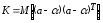
матрицу К,
являющуюся
матричным аналогом дисперсии одной
переменной:
 .
.
где
элементы
 ковариации
(или
корреляционные
моменты) оценок
параметров
 и
и
 .
.
Ковариация
двух переменных определяется как
математическое ожидание произведения
отклонений этих переменных от их
математических ожиданий [Ссылка]. Поэтому
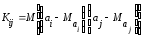 , (13.28)
где
 и
и математические
ожидания соответственно для параметров
и
 .
.
Ковариация
характеризует как степень рассеяния
значений двух переменных относительно
их математических ожиданий, так и
взаимосвязь этих переменных.
В
силу того, что оценки
 ,
,
полученные методом наименьших квадратов,
являются несмещенными оценками параметров ,
,
т.е.
 ,
,
выражение(13.28)
примет
вид:
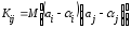 .
.
Рассматривая
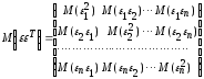
ковариационную матрицу К,
легко
заметить, что на ее главной диагонали
находятся дисперсии опенок параметров
регрессии, ибо
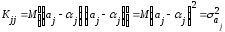 .
.
(13.29)
В
сокращенном виде ковариационная матрица
К
имеет
вид:
 .
.
(13.30)
Учитывая
(13.28)
мы
можем записать
 .
.
Тогда
выражение (12.30) примет вид:
 ,
,
(13.31)
ибо
элементы матрицы X
—неслучайные
величины.
Матрица

представляет
собой ковариационную матрицу
вектора возмущений
 :
:
в
которой все элементы, не лежащие на
главной диагонали, равны нулю в силу
предпосылки 4
о
некоррелированности возмущений
 ,
,
и
между
собой,
а
все элементы, лежащие на главной
диагонали, в силу предпосылок 2
и
3
регрессионного
анализа
равны
одной и той же дисперсии
 :
:
 .
.
Поэтому
матрица
 ,
,
где

единичная
матрица
 го
го
порядка.
Следовательно, в силу (13.31)
ковариационная
матрица вектора

оценок
параметров:

Так
как
 и
и
 ,
,
то окончательно получим:
 (13.32)
Таким
образом, с
помощью обратной матрицы нормальных
уравнении регрессии
определяется
не только сам вектор
 оценок
параметров (13.28),
но
и дисперсии и ковариации его компонент.
Входящая
в (13.32)
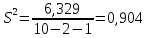
дисперсия
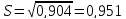
возмущений неизвестна. Заменив ее
выборочной остаточной дисперсией
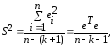 (13.33)
по
(13.32)
получаем
выборочную оценку ковариационной
матрицы К.
(В
знаменателе выражения (13.33)
стоит
 ,
,
а
не
 ,
,
как
это было выше в (13.6).
Это
связано с тем, что теперь
 степеней
свободы (а не две) теряются при определении
неизвестных параметров, число которых
вместе со свободным членом равно
равно .
.
4.10. Определение доверительных интервалов для коэффициентов и функции множественной регрессии
Перейдем
теперь к оценке значимости коэффициентов
регрессии

и
построению доверительного интервала
для параметров регрессионной модели
 .
.
В
силу (13.29),
(13.32) и
изложенного выше оценка дисперсии
коэффициента регрессии

определится
по формуле:

где

несмещенная
оценка параметра
 ;
;
 диагональный
элемент матрицы
 .
.
Среднее
квадратическое отклонение (стандартная
ошибка) коэффициента регрессии

примет
вид:
 .
.
(13.34)
Значимость
коэффициента регрессии

можно
проверить, если учесть, что статистика
 имеет
имеет распределение
Стьюдента с
 степенями
свободы. Поэтому

значимо
отличается от нуля на уровне
значимости
 ,
,
если соответствующий
 ныйдоверительный
интервал для параметра

есть
 .
.
(13.35)
Наряду
с интервальным оцениванием коэффициентов
регрессии по (13.35)
весьма
важным для оценки точности определения
зависимой переменной (прогноза) является
построение доверительного
интервала для функции регрессии или
для условного математического
ожидания зависимой переменной
 ,
,
найденного в предположении, что
объясняющие переменные
приняли
значения, задаваемые вектором
 .Выше
.Выше
такой интервал получен для уравнения
парной регрессии (см. (13.13)
и
(13.12)).
Обобщая
соответствующие выражения на случай
множественной регрессии, можно получить
доверительный интервал для
 :
:
где
 групповая
средняя, определяемая по уравнению
регрессии,
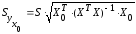 (13.36)
— ее
стандартная ошибка.
При
обобщении формул (13.15)
и
(13.14)
аналогичный
доверительный
интервал для индивидуальных значений
зависимой переменной
 примет
вид:
 (13.37)
где
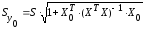 .
.
(13.38)
Доверительный
интервал для дисперсии возмущений

в
множественной регрессии с надежностью
 строится аналогично парной модели
по формуле(13.20)
с
соответствующим изменением числа
степеней свободы критерия
 :
:
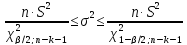 (13.39)
Пример
13.6.
По
данным примера 13.4
оценить
сменную добычу
угля на одного рабочего для шахт с
мощностью пласта 8 м и уровнем механизации
работ 6%; найти 95%-ные доверительные
интервалы для индивидуального и среднего
значений сменной добычи угля на 1
рабочего для таких же шахт. Проверить
значимость коэффициентов регрессии и
построить для них 95%-ные доверительные
интервалы. Найти с надежностью 0,95
интервальную оценку для дисперсии
возмущений
 .
.
Решение.
В примере 13.4
уравнение
регрессии получено в виде:
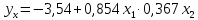 .
.
По
условию надо оценить
 ,
,
где
 .
.
Выборочной оценкой ,
,
является
групповая средняя, которую найдем по
уравнению регрессии:
 .
.
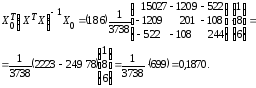
Для построения доверительного
интервала для М (у) необходимо знать
дисперсию его оценки .
.
Для
ее вычисления обратимся к табл. 13.7
(точнее к ее двум последним столбцам,
при составлении которых учтено, что
групповые средние определяются по
полученному уравнению регрессии).
Теперь
по (13.37):
и
 (т).
(т).
Определяем
стандартную ошибку групповой средней
г> по формуле (13.41).
Вначале
найдем
Теперь
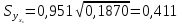
(т).
По
табл. IV приложений при числе степеней
свободы
находим
 .
.
По
(13.40)
доверительный
интервал для
 ,
,
равен
 или
или (т).
(т).
Итак,
с надежностью 0,95
средняя
сменная добыча угля на одного рабочего
для шахт с мощностью пласта 8
м
и уровнем механизации работ 6%
находится
в пределах от 4,52
до
6,46
т.
Сравнивая
новый доверительный интервал для функции
регрессии
 ,
,
полученный
с учетом двух объясняющих переменных,
с аналогичным интервалом с учетом одной
объясняющей переменной (см. пример
13.1),
можно
заметить уменьшение его величины. Это
связано с тем, что включение в модель
новой объясняющей переменной позволяет
несколько повысить точность модели
за счет увеличения взаимосвязи зависимой
и объясняющей переменных (см. ниже).
Найдем
доверительный интервал для индивидуального
значения

при
 по
по
(13.43):

(т)
и по (13.42):
 ,
,
т. е.
 (т).
(т).
Итак,
с надежностью 0,95
индивидуальное
значение сменной добычи угля в шахтах
с мощностью пласта 8
м
и уровнем механизации работ 6%
находится
в пределах от 3,05
до
7,93
(т).
Проверим
значимость коэффициентов регрессии

и
 .
.
В
примере 13.4
получены

и
 .
.
Стандартная
ошибка

в
соответствии с (13.38)
равна:
 .
.
Так
как
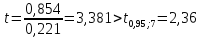 ,
,
то
коэффициент

значим.
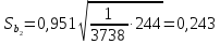
Аналогично вычисляем
 и
и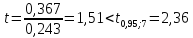 т.е. коэффициент
незначим
на 5%-ном уровне.
Доверительный
интервал имеет смысл построить только
для значимого коэффициента регрессии
 :
:
по
(13.39)

или
 .
.
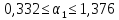
Итак,
с надежностью 0,95 за счет изменения на
1 м мощности пласта

(при
неизменном
 )
)
сменная
добыча угля на одного рабочего У
будет изменяться в пределах от 0,332 до
1,376 т.
Найдем
95%-ный доверительный интервал для
параметра ст2.
Учитывая, что
 ,
, ,
, найдем по табл.
V
приложений при
 степенях свободы
 ;
; и по формуле(13.43′)

Таким
образом, с надежностью 0,95 дисперсия
возмущений заключена в пределах от
0,565 до 5,35, а их стандартное отклонение
— от 0,751 до 2,31 (т).
Формально
переменные, имеющие незначимые
коэффициенты регрессии, могут быть
исключены из рассмотрения. В экономических
исследованиях исключению переменных
из регрессии должен предшествовать
тщательный качественный
анализ.
Поэтому может оказаться целесообразным
все же оставить в регрессионной модели
одну или несколько объясняющих
переменных, не оказывающих существенного
(значимого) влияния на зависимую
переменную.
Соседние файлы в предмете [НЕСОРТИРОВАННОЕ]
- #
- #
- #
- #
- #
27.03.20162.81 Mб141Учебник Туристское ресурсоведение.rtf
- #
- #
- #
- #
- #
- #
27.03.20164.24 Mб198Физика Яковлев.pdf
Вариации
оценок параметров будут, в конечном
счете, определять точность уравнения
множественной регрессии. Для их измерения
в многомерном регрессионном анализе
рассматривают так называемую
ковариационную
матрицу К,
являющуюся
матричным аналогом дисперсии одной
переменной:
.
где
элементы
ковариации
(или
корреляционные
моменты) оценок
параметров
и.
Ковариация
двух переменных определяется как
математическое ожидание произведения
отклонений этих переменных от их
математических ожиданий [Ссылка]. Поэтому
, (13.28)
где
иматематические
ожидания соответственно для параметров
и
.
Ковариация
характеризует как степень рассеяния
значений двух переменных относительно
их математических ожиданий, так и
взаимосвязь этих переменных.
В
силу того, что оценки
,
полученные методом наименьших квадратов,
являются несмещенными оценками параметров,
т.е.
,
выражение(13.28)
примет
вид:
.
Рассматривая
ковариационную матрицу К,
легко
заметить, что на ее главной диагонали
находятся дисперсии опенок параметров
регрессии, ибо
.
(13.29)
В
сокращенном виде ковариационная матрица
К
имеет
вид:
.
(13.30)
Учитывая
(13.28)
мы
можем записать
.
Тогда
выражение (12.30) примет вид:
,
(13.31)
ибо
элементы матрицы X
—неслучайные
величины.
Матрица
представляет
собой ковариационную матрицу
вектора возмущений
:
в
которой все элементы, не лежащие на
главной диагонали, равны нулю в силу
предпосылки 4
о
некоррелированности возмущений
,
и
между
собой,
а
все элементы, лежащие на главной
диагонали, в силу предпосылок 2
и
3
регрессионного
анализа
равны
одной и той же дисперсии
:
.
Поэтому
матрица
,
где
единичная
матрица
го
порядка.
Следовательно, в силу (13.31)
ковариационная
матрица вектора
оценок
параметров:
Так
как
и
,
то окончательно получим:
(13.32)
Таким
образом, с
помощью обратной матрицынормальных
уравнении регрессии
определяется
не только сам вектор
оценок
параметров (13.28),
но
и дисперсии и ковариации его компонент.
Входящая
в (13.32)
дисперсия
возмущений неизвестна. Заменив ее
выборочной остаточной дисперсией
(13.33)
по
(13.32)
получаем
выборочную оценку ковариационной
матрицы К.
(В
знаменателе выражения (13.33)
стоит
,
а
не
,
как
это было выше в (13.6).
Это
связано с тем, что теперь
степеней
свободы (а не две) теряются при определении
неизвестных параметров, число которых
вместе со свободным членомравно.
4.10. Определение доверительных интервалов для коэффициентов и функции множественной регрессии
Перейдем
теперь к оценке значимости коэффициентов
регрессии
и
построению доверительного интервала
для параметров регрессионной модели
.
В
силу (13.29),
(13.32) и
изложенного выше оценка дисперсии
коэффициента регрессии
определится
по формуле:
где
несмещенная
оценка параметра
;
диагональный
элемент матрицы
.
Среднее
квадратическое отклонение (стандартная
ошибка) коэффициента регрессии
примет
вид:
.
(13.34)
Значимость
коэффициента регрессии
можно
проверить, если учесть, что статистика
имеетраспределение
Стьюдента с
степенями
свободы. Поэтому
значимо
отличается от нуля на уровне
значимости
,
еслисоответствующийныйдоверительный
интервал для параметра
есть
.
(13.35)
Наряду
с интервальным оцениванием коэффициентов
регрессии по (13.35)
весьма
важным для оценки точности определения
зависимой переменной (прогноза) является
построение доверительного
интервала для функции регрессии или
для условного математического
ожидания зависимой переменной
,
найденного в предположении, что
объясняющие переменные
приняли
значения, задаваемые вектором
.Выше
такой интервал получен для уравнения
парной регрессии (см. (13.13)
и
(13.12)).
Обобщая
соответствующие выражения на случай
множественной регрессии, можно получить
доверительный интервал для
:
где
групповая
средняя, определяемая по уравнению
регрессии,
(13.36)
— ее
стандартная ошибка.
При
обобщении формул (13.15)
и
(13.14)
аналогичный
доверительный
интервал для индивидуальных значений
зависимой переменной
примет
вид:
(13.37)
где
.
(13.38)
Доверительный
интервал для дисперсии возмущений
в
множественной регрессии с надежностью
строится аналогично парной модели
по формуле(13.20)
с
соответствующим изменением числа
степеней свободы критерия
:
(13.39)
Пример
13.6.
По
данным примера 13.4
оценить
сменную добычу
угля на одного рабочего для шахт с
мощностью пласта 8 м и уровнем механизации
работ 6%; найти 95%-ные доверительные
интервалы для индивидуального и среднего
значений сменной добычи угля на 1
рабочего для таких же шахт. Проверить
значимость коэффициентов регрессии и
построить для них 95%-ные доверительные
интервалы. Найти с надежностью 0,95
интервальную оценку для дисперсии
возмущений
.
Решение.
В примере 13.4
уравнение
регрессии получено в виде:
.
По
условию надо оценить
,
где
.
Выборочной оценкой,
является
групповая средняя, которую найдем по
уравнению регрессии:
.
Для построения доверительного
интервала для М (у) необходимо знать
дисперсию его оценки.
Для
ее вычисления обратимся к табл. 13.7
(точнее к ее двум последним столбцам,
при составлении которых учтено, что
групповые средние определяются по
полученному уравнению регрессии).
Теперь
по (13.37):
и
(т).
Определяем
стандартную ошибку групповой средней
г> по формуле (13.41).
Вначале
найдем
Теперь
(т).
По
табл. IV приложений при числе степеней
свободы
находим
.
По
(13.40)
доверительный
интервал для
,
равен
или(т).
Итак,
с надежностью 0,95
средняя
сменная добыча угля на одного рабочего
для шахт с мощностью пласта 8
м
и уровнем механизации работ 6%
находится
в пределах от 4,52
до
6,46
т.
Сравнивая
новый доверительный интервал для функции
регрессии
,
полученный
с учетом двух объясняющих переменных,
с аналогичным интервалом с учетом одной
объясняющей переменной (см. пример
13.1),
можно
заметить уменьшение его величины. Это
связано с тем, что включение в модель
новой объясняющей переменной позволяет
несколько повысить точность модели
за счет увеличения взаимосвязи зависимой
и объясняющей переменных (см. ниже).
Найдем
доверительный интервал для индивидуального
значения
при
по
(13.43):
(т)
и по (13.42):
,
т. е.
(т).
Итак,
с надежностью 0,95
индивидуальное
значение сменной добычи угля в шахтах
с мощностью пласта 8
м
и уровнем механизации работ 6%
находится
в пределах от 3,05
до
7,93
(т).
Проверим
значимость коэффициентов регрессии
и
.
В
примере 13.4
получены
и
.
Стандартная
ошибка
в
соответствии с (13.38)
равна:
.
Так
как
,
то
коэффициент
значим.
Аналогично вычисляем
ит.е. коэффициент
незначим
на 5%-ном уровне.
Доверительный
интервал имеет смысл построить только
для значимого коэффициента регрессии
:
по
(13.39)
или
.
Итак,
с надежностью 0,95 за счет изменения на
1 м мощности пласта
(при
неизменном
)
сменная
добыча угля на одного рабочего У
будет изменяться в пределах от 0,332 до
1,376 т.
Найдем
95%-ный доверительный интервал для
параметра ст2.
Учитывая, что
,,найдем по табл.
V
приложений при
степенях свободы;и по формуле(13.43′)
Таким
образом, с надежностью 0,95 дисперсия
возмущений заключена в пределах от
0,565 до 5,35, а их стандартное отклонение
— от 0,751 до 2,31 (т).
Формально
переменные, имеющие незначимые
коэффициенты регрессии, могут быть
исключены из рассмотрения. В экономических
исследованиях исключению переменных
из регрессии должен предшествовать
тщательный качественный
анализ.
Поэтому может оказаться целесообразным
все же оставить в регрессионной модели
одну или несколько объясняющих
переменных, не оказывающих существенного
(значимого) влияния на зависимую
переменную.
Соседние файлы в предмете [НЕСОРТИРОВАННОЕ]
- #
- #
- #
- #
- #
27.03.20162.81 Mб141Учебник Туристское ресурсоведение.rtf
- #
- #
- #
- #
- #
- #
27.03.20164.24 Mб196Физика Яковлев.pdf
Battery state-of-power evaluation methods
Shunli Wang, … Zonghai Chen, in Battery System Modeling, 2021
7.4.4 Main charge-discharge condition test
The initial value of the error covariance matrix P0 can be determined from the X0 error of the initial state. In the application, the initial value should be as small as possible to speed up the tracking speed of the algorithm. Two important parameters are processed noise variance matrix Q and observation noise variance matrix R. As can be known from theoretical formula derivation, the dispose to Q and R plays a key role in improving the estimation effect by using this algorithm. Because it affects the size of the Kalman gain matrix K directly, the value of error covariance matrix P can be described as shown in Eq. (7.61):
(7.61)Rk=Eυk2=συ2
It is the expression of the observation noise variance, which is mainly derived from the distribution of observation error of experimental instruments and sensors, as shown in Eq. (7.62):
(7.62)Qk=Eω1k2Eω1kω2kEω2kω1kEω2k2=σω1,12σω1,22σω2,12σω2,22
It is the relationship between the system noise variance and the processing noise covariance. The two states in the system are generally unrelated and the covariance value is zero. Therefore, the diagonal variance can have a small value. The variance Q of processing noise is mainly derived from the error of the established equivalent model, which is difficult to be obtained by theoretical methods or means. A reasonable value range can be obtained through continuous debugging through simulation, and it is usually a small amount.
To verify the applicable range and stability of the algorithm, the input of different working conditions is used to observe the estimation accuracy of the algorithm. In this simulation, two working conditions are used: the constant-current working condition and the Beijing bus dynamic street test working condition. For the constant-current condition, only a constant value needs to be set in the program. To increase the complexity of the condition, two shelved stages are added to the constant-current input list to verify the tracking effect of Ah and the extended Kalman filtering. The following code is generated for the current.
The experimental data should be used to simulate the algorithm under its operating conditions. The current input module is realized in the environment under Beijing bus dynamic street test operating conditions. It is the time integration module, whose output is the capacity change of the working condition, and the lower part is the working condition data output module. It outputs the current into the workspace at the minimum time interval of the sampling measurement. The data onto the workspace are a time-series type and the current data need to be extracted. The data extraction and transformation can be performed in the main program, wherein the working condition is the Simulink module. The current is the time-series data, including the current output. S_Est is the algorithm program module, whose input is the initial S_Est_init and current data onto the estimated state value.
The current data are input into the program module of the extended Kalman filtering algorithm based on the model, and the initial values of other parameters have been determined in the program. The program finally outputs the ampere hour time integral and the state estimation curve of the extended Kalman filtering through the minimum time interval of 10 times as the sampling time. The current curve of the experimental test can be obtained as shown in Fig. 7.13.

Fig. 7.13. Pulse current operating current curve for the experimental test. (A) Main charge working condition. (B) Main discharge experimental test.
The unscented Kalman filtering algorithm is programmed by writing scripts to realize algorithm simulation to compare the output effect. The specific implementation process conforms to the processing requirements, and the main simulation program can be constructed. The program takes 10 times the minimum time interval as the sampling time and simulates the three methods of the state estimation, including ampere hour time integration, extended Kalman filtering, and unscented Kalman filtering, to compare the following situation of the three methods of the state over time. The program simultaneously outputs the state variation curve and estimation error curve with time, so that the tracking effect and error variation on the three methods can be obtained visually. Its implementation process is consistent with script. Different modules are used to replace the code block. The integration advantage of the environment is used in the graphical interface to obtain the same stimulation effect.
The operation logic is ensured by the unchanged intuitive presentation of the calculation process. Based on script implementation, the modular simulation is built accordingly. The experiment data are used as the input current, and the state prediction is obtained by the state prediction module. The forecast and model parameters are calculated. After that, the equivalent model can be used to predict the completion status value of Up as well as the output voltage. The input of the algorithm includes the update module, output state correction, and error covariance matrix update as the basis of the forecast. It takes the ampere hour integral result as the minimum time interval of the current data, which is taken as the reference value of the measured state.
The estimation effect of ampere hour and extended Kalman filtering is compared when the minimum time interval can be set as 10 times as the sampling period. The stability of the extended Kalman filtering algorithm is evaluated under working conditions. The state variable needs to accept the last estimated value as the basis of the next state prediction, in which the predicted value Up_pre is directly input into the corresponding position of the resistance-capacitance circuit modeling to conduct the terminal voltage prediction of the current polarization voltage. The functions of each part are realized in a more modular way for the complete structure and clear hierarchy.
Read full chapter
URL:
https://www.sciencedirect.com/science/article/pii/B9780323904728000044
Dynamic Model Development
P.W. Oxby, … T.A. Duever, in Computer Aided Chemical Engineering, 2003
3.2 An Optimality Property of the Determinant Criterion
Equation (12) can be generalized by replacing the inverse of the estimate of the error covariance matrix,
Σ^εn−1, with an arbitrary symmetric positive definite weight matrix, W:
(14)Δθ^(k)=(XTWX)−1XTWz(θ^(k))
The estimate of the parameter covariance is:
(15)Σ^θ=(XTWX)−1XTWΣ^εn(XTWX)−1
If the determinant of the estimate of the parameter covariance matrix,
|Σ^θ|, is minimized with respect to the elements of W, the solution is independent of X and is simply
(16)W=Σ^εn−1
Substitution of (16) back into (14) gives (12) which, as has been shown, is equivalent to the determinant criterion. Therefore of all weighting schemes in the form of (14), it is the one equivalent to the determinant criterion that minimizes
|Σ^θ|, the determinant of the estimate of the parameter covariance matrix when the error covariance is unknown. This appears to be a rather strong result in support of the determinant criterion. It might also be noted that, unlike derivations based on likelihood, this result does not depend on the measurement errors being normally distributed. But it will be shown that the practical usefulness of the result does depend on the assumption that the residual covariance
Z(θ^)Z(θ^)T/n, is a good estimate of the true error covariance. Ideally one would want W to be the inverse of the error covariance matrix. The determinant in effect makes a compromise and substitutes an estimate of it. The potential problem here is that if the data set is not large, the residual covariance matrix may be a poor estimate of the error covariance matrix. A poor estimate of the error covariance matrix will lead to a poor estimate of the parameter covariance matrix. Therefore, although the determinant criterion gives the minimum determinant of the estimate of the parameter covariance matrix, if this estimate is poor, then the optimality property may be of little significance. This suggests that the optimality of the determinant criterion may be more relevant for large data sets than small ones. The simulation studies presented in Section 4 will confirm this to be true.
Read full chapter
URL:
https://www.sciencedirect.com/science/article/pii/S1570794603800706
Kalman Filters and Nonlinear Filters
Vytas B. Gylys, in Encyclopedia of Physical Science and Technology (Third Edition), 2003
IV.B Square Root Filtering
By far the greatest trouble spot in computer mechanization of the KF is the updating of state error covariance matrix P, that is, the computation of Pk∣k according to Eq. (18). As the estimation process progresses, the elements of Pk∣k typically continue to decrease in magnitude and so matrix Pk∣k keeps approaching the zero matrix, although theoretically it should forever remain positive definite, no matter how small in magnitude its elements become. Hence, unless special measures are taken, accumulation of roundoff error in the repetitive use of Eq. (18) may cause the computed Pk∣k to lose its positive definiteness. As suggested by the matrix inversion operation appearing on the right-hand side of Eq. (16) for computing the Kalman gain, this situation is aggravated if several components of the measurement vector are very accurate and consequently the positive definite measurement error covariance matrix R is ill conditioned, that is, if R has eigenvalues of both relatively very large and small magnitudes.
Let A be a nonnegative definite symmetric matrix; then there exists a matrix S such that A = SST. Matrix S is often called the square root of A. The Cholesky decomposition algorithm provides a method of constructing from A the matrix S so that S is lower triangular; that is, all elements of S above the main diagonal are zero. Square root filtering is motivated by the observations that, if the state error covariance matrix P = SST, then (a) since SST is always nonnegative definite, matrix P expressed as SST cannot become negative definite, and (b) matrix S is generally less ill conditioned than matrix P.
Several versions of the square root filtering algorithm are known. The earliest form was developed by J. E. Potter in 1964 for applications in which the process noise is absent (i.e., covariance matrix Q is zero) and the measurements are sequentially processed as scalars. In 1967 J. F. Bellantoni and K. W. Dodge extended Potter’s results to vector-valued measurements. A. Andrews in 1968 and then S. F. Schmidt in 1970 published two alternative procedures for handling the process noise. In 1973 N. A. Carlson described a procedure that considerably improved the speed and decreased the memory requirements of square root filtering and in which, as in Potter’s algorithm, vector-valued measurements are processed sequentially as scalars. Finally, the so-called UDUT covariance factorization method is the most recent major milestone in numerical handling of KFs. This method, developed by G. J. Bierman and C. L. Thornton, represents the state error covariances before and after the measurement update step asPk|k−1=Uk|k−1Dk|k−1Uk|k−1TandPk|k=Uk|kDk|kUk|kT,with D being a diagonal matrix and U an upper triangular matrix with 1’s on its main diagonal. In this method, the square root of the covariance matrix, which now would correspond to UD1/2, is never computed explicitly, which avoids numerical computation of square roots. Like Carlson’s algorithm, the UDUT factorization method maintains the covariance matrix in factored form and so (like Carlson’s algorithm) is considerably more efficient in processor time and storage than the original Potter algorithm.
As a quick comparison of computational efficiency, the conventional Kalman method, the less efficient form of Carlson’s algorithm, and the UDUT factorization method are roughly equal: The processing of each time step (consisting of one time propagation and one measurement update) requires of the order of 16[9ns3 + 9ns2nm + 3ns2nw] adds and about the same number of multiplies, plus a relatively modest number of divides and square roots (square roots are required only in some, as in Potter’s or Carlson’s square root algorithms). Here, as before, ns is the length of the state vector, nm the length of the measurement vector, and nw the lenght of the process noise vector w. The faster version of Carlson’s algorithm is more efficient and requires only of the order of 16[5ns3 + 9ns2nm + 3ns2nw] adds and 16[5ns3 + 12ns2nm + 3ns2nw] multiplies, plus 2nsnm divides and nsnm square roots, at each time point. The stable (Joseph) form of the KF [as given by Eq. (18′)] fares more poorly: At each time step, it requires of the order of 16[18ns3 + 15ns2nm + 3ns2nw] adds and about the same number of multiplies.
As a summary, (a) a square root filter is a numerically stable form for performing the KF covariance–gain processing defined by Eqs. (15), (16), and (18); (b) the efficiency of its more recent versions roughly compares with that of these three equations; (c) the increased stability allows one to use relatively low-precision arithmetic in the KF gain–covariance processing, with a possible exception of some dot products.
Real-time implementation of a filter involves additional issues that are unimportant in the non-real-time environment. Besides the adequacy of functional performance, the most important of these issues is the requirement to produce timely responses to external stimuli. Thus, resorting to a parallel or concurrent processing may be the only way out. This usually implies the use of special hardware architectures such as parallel, vector pipelined, or systolic processors.
As one example, consider the use of a filter in the tracking of multiple objects in a hard real-time environment characterized by strict deadlines. In such a case one may want to maintain simultaneously many estimation processes, each handling a single object. Parallel processors may seem to be a suitable hardware architecture for this problem, but if separate estimation processes in such an application progress at different rates and at any time some of them require a great amount of special handling, then parallel architecture, such as a single-instruction multiple-data stream computer, may not be the best choice. As another example, consider a KF to be implemented as part of a navigation system on a small airborne computer (uniprocessor). Suppose that the navigation measurements come at a certain fixed rate. If the filtering process cannot keep up with the arrival rate of measurements and so not all of them can be utilized, the estimation performance may deteriorate. In this problem, if there is an upper bound on hardware resources, the only solution may be to decompose the estimation algorithm into concurrently executable processes. For instance, the time-propagation step (which, say, is to be executed at a relatively high rate) may constitute one process and the measurement-update step (which needs to be executed only at some lower rate, say, at the rate of measurement arrivals) may constitute another. Such a decomposition of an estimation algorithm into concurrent procedures often creates a surrogate algorithm that performs more poorly than the original algorithm.
The effects of the finite-length word computing is another issue that must be considered in filter implementation for real-time applications. The computer on which a filter is developed and validated through successive off-line simulations is often more powerful and uses higher-precision arithmetic and number representations than the ultimate real-time processor. Hence, one must in advance determine in advance what effect a shorter word length will have on performance.
Read full chapter
URL:
https://www.sciencedirect.com/science/article/pii/B0122274105003574
Computer Techniques and Algorithms in Digital Signal Processing
K. Giridhar, … Ronald A. Iltis, in Control and Dynamic Systems, 1996
A Appendix – Time Updates for the Blind MAPSD Algorithm
In this Appendix, we derive the one-step time updates of the channel estimate and the associated error covariance matrix for the blind MAP symbol detector developed in Section 4.2. Recall from Eq. (51) that
(A.1)pfk+1|dik+1,Nf,rk=∑j:djk,Nf∈dik+1,Nfαjp(fk+1|djk,Nf,rk)
where αj is given by Eq. (52). Using Eq. (49), this Gaussian sum can be explicitly written as follows:
(A.2)pfk+1|dik+1,Nf,rk=∑j:djk,Nf∈dik+1,NfαjNfk+1;Ff^jk|k,FPjk|kFH+Q
which defines the one-step prediction of the mean vector f^ik+1|k and the covariance matrix Pik+1|k. Some basic results about sums of Gaussian p.d.f.s can be used to derive these one-step predictions.
Lemma: Let the p.d.f. of the random vector x be a weighted sum of N multivariate Gaussian p.d.f.s as follows:
(A.3)px=∑j=1NαjNx;xj,Pj
where αj , xj, and Pj are, respectively, the jth weight, mean, and covariance. (i) The mean value of x is given by
(A.4)xa=∑j=1Nαjxj.
(ii) The error covariance is given by
(A.5)Pa=∑j=1NαjPj+xa–xjxa–xjH.
Proof: The first part of the lemma is easily proved from the definition of xa, i.e.,
(A.6)xa=Ex=∫xx∑j=1NαjNx;xj,Pjdx=∑j=1Nαjxj.
To prove the second part of the lemma, consider
(A.7)Pa=Ex−xax−xaH=∑j=1Nαj∫xxxHNjdx+xaxaH−∫xxxaHNjdx−∫xxaxHNjdx
where, for convenience, we have used the notation Nj to represent the p.d.f. N(x; xj, Pĵ). Observe that ∫xxaHNjdx=xjxaHand∫xaxHNjdx=xaxjH. By adding and subtracting the term xjxjH to the expression inside the square brackets, we obtain
(A.8)Pa=∑j=1Nαj∫xxxHNjdx−xjxjH+xaxaH−xjxaH−xaxjH+xjxjH=∑j=1Nαj∫xxxHNjdx−xjxjH+xa−xjxa−xjH..
It is straightforward to show that
(A.9)∑j=1Nαj∫xxxHNjdx−xjxjH=∑j=1Nαj∫xx−xj(x−xj)HNjdx=∑j=1NαjPj.
Substituting this result into Eq. (A.8 ), we obtain the result in Eq. (A.5 ) for the error covariance Pa, which completes the proof.
To obtain the one-step predicted mean vector of the blind MAPSD algorithm, Eq. (A.4 ) is used with xj=Ff^jk|k. The summation is performed over the M predecessor subsequences djk,Nf, yielding
(A.10)f^ik+1|k)=∑j:djk,Nf∈dik+1,NfαjFf^jk|k.
By substituting αj=pdjk,Nf|rk−1/qik, the final expression in Eq. (53) is obtained. Similarly, the one-step error covariance update in Eq. (54) is obtained by substituting FPjk|kFH+Q=Pj and
(A.11)νj,ikνj,iHk=xa−xjxa−xjH
into Eq. (A.5 ) where xa=f^ik+1|k (and xj=Ff^jk|k as above).
Read full chapter
URL:
https://www.sciencedirect.com/science/article/pii/S0090526796800454
State Estimation
Jay Farrell, in The Electrical Engineering Handbook, 2005
4.3 Recursive State Estimation
Equations 4.4 through 4.5 provide the mean and the covariance of the state through time based only on the initial mean state vector and its error covariance matrix. When measurements y(k) are available, the measurements can be used to improve the accuracy of an estimate of the state vector at time k. The symbols xˆ−(k) and xˆ+(k) are used to denote the estimate of x(k) before and after incorporating the measurement, respectively.
Similarly, the symbols Pxˆ−(k) and Pxˆ+(k) are used to denote the error covariance matrices corresponding to xˆ−(k) and xˆ+(k), respectively. This section presents the time propagation and measurement update equations for both the state estimate and its error covariance. The equations are presented in a form that is valid for any linear unbiased measurement correction. These equations contain a gain matrix K that determines the estimator performance. The choice of K to minimize the error covariance Pxˆ+(k) will be of interest.
For an unbiased linear measurement, the update will have the form:
(4.8)xˆ+(k)=xˆ−(k)+K(k)(y(k)−yˆ−(k)),
where yˆ−(k)=H(k)xˆ−(k).. The error covariance of xˆ+(k) is the following:
(4.9)Pxˆ+(k)=(I−K(k)H(k))Pxˆ−(k)(I−K(k)H(k))T +K(k)R(k)KT(k).
K(k) is a possibly time-varying state estimation gain vector to be designed. If no measurement is available at time k, then K(k) = 0, which yields xˆ+(k)=xˆ−(k) and Pxˆ+(k)=Pxˆ−(k). If a measurement is available, and the state estimator is designed well, then Pxˆ+(k)≤Pxˆ−(k). In either case, the time propagation of the state estimate and its error covariance matrix is achieved by:
(4.10)xˆ−(k+1)=Φ(k)xˆ+(k)+Γˆuu(k)
(4.11)Pxˆ−(k+1)=Φ(k)Pxˆ+(k)ΦT(k)+ΓωQd(k)ΓωT.
At least two issues are of interest relative to the state estimation problem. First, does there exist a state estimation gain vector K(k) such that xˆ is guaranteed to converge to x regardless of initial condition and the sequence u(k)? Second, how should the designer select the gain vector K(k)?
The first issue raises the question of observability. A linear time-invariant system is observable if the following matrix has rank n:
[HT, ΦTHT, …,( ΦT)nHT].
When a system is observable, then it is guaranteed that a stabilizing gain vector K exists. Assuming that the system of interest is observable, the remainder of this chapter discusses the design and analysis of state estimators.
Figure 4.1 portrays the state estimator in conjunction with the system of interest. The system of interest is depicted in the upper left. The state estimator is superimposed on a gray background in the lower right.

FIGURE 4.1. State Estimation System Block Diagram
This interconnected system will be referred to as the state estimation system. The figure motivates several important comments. First, although the state estimator has only n states, the state estimation system has 2n states. Second, the inputs to the state estimation system are the deterministic input u and the stochastic inputs ω and v. Third, the inputs to the state estimator are the deterministic input u and the measured plant output y. The state space model for the state estimation system is the following:
(4.12)[x(k+1)xˆ−(k+1)]=[Φx0LHxΦ−LH][x(k)xˆ−(k)]+[ΓuΓω0Γˆu0L][u(k)ω(k)v(k)],
where L = ΦK.
Based on this state-space model, with the assumption that the system is time invariant, the transfer function from v to yˆ is as written here:
(4.13)Gv(z)=H[zI−(Φ−LH)]−1L,
where z is the discrete-time unit advance operator. Assuming that H = Hx, the transfer function from u to r is as follows:
(4.14)Gu(z)=H[zI−(Φ−LH)]−1 [(zI−Φ)(zI−Φx)−1Γu−(zI−Φx)(zI−Φx)−1Γˆu].
Therefore, if Γu=Γˆu and Φx = Φ, then this transfer function is identically zero. Assuming again that H = Hx, the transfer function from ω to r is the following:
(4.15)Gω(z)=H[zI−(Φ−LH)]−1[zI−Φ][zI−Φx]−1Γω.
In the special case where, in addition, Φx = Φ, the transfer function Gω(z) has n identical poles and zeros. This transfer functions is often stated as:
(4.16)Gω(z)=H[zI−(Φ−LH)]−1Γω,
where n pole and zero cancellations have occurred. These pole-zero cancellations and therefore the validity of equation 4.16 are dependent on the exact modeling assumption and the stability of the canceled poles.
Read full chapter
URL:
https://www.sciencedirect.com/science/article/pii/B9780121709600500815
Data Assimilation in Numerical Weather Prediction and Sample Applications
Andrew S. Jones, Steven J. Fletcher, in Solar Energy Forecasting and Resource Assessment, 2013
13.3.5 Ensemble DA
The ensemble Kalman filter (EnsKF) is a sequential filter that forecasts the state vector, xf, as well as the model-error covariance matrix, Pf, toward a future time step (Evensen, 1994). This is a linear process, but it can employ nonlinear models within the system; no adjoints are required. For example, the forward state is given by the propagation of the model forward in time
(13.29)xf(ti)=Mi−1[xa(ti−1)]
as well as its associated forecast-error covariance matrix
(13.30)Pf(ti)=Mi−1Pa(ti−1)Mi−1T+Q(ti−1)
This is followed by an analysis step that updates (or readjusts) the state information and the forecast-error covariance information
(13.31)xa(ti)=xf(ti)+Kidi
(13.32)Pa(ti)=(I−KiHi)Pf(ti)
where the innovation vector, di, is given by
(13.33)di=yio−Hi[xf(ti)]
It is important to note that M and H are linearizations of the gradients of M and H with respect to the control vector, x. The Kalman gain, Ki, is given by
(13.34)Ki=Pf(ti)HiT[HiPf(ti)HiT+Ri]−1
where Pf(ti) is now approximated by the mean ensemble estimate
(13.35)Pf(ti)≈1K−2∑K≠lK[xf(tk)−x¯f(tl)][xf(tk)−x¯f(tl)]T
K is the number of ensemble-model runs required to generate the estimate, and a reference model state, l, is used to define the mean ensemble estimate of the forecast error covariance matrix. In addition to the approach in equation 13.35, other EnsKF variants are used by the NWP DA community. The analysis stage that propagates the forecast error covariance matrix is a powerful feature of EnsKF. Additional improvements in EnsKF performance can be achieved by improving sampling behaviors—for example, using sampling strategies and square root schemes, some of which also allow for a low-rank representation of the observational-error covariance matrix (Evensen, 2004).
Read full chapter
URL:
https://www.sciencedirect.com/science/article/pii/B9780123971777000139
The Basics of Analytical Mechanics, Optimization, Control and Estimation
Kyle T. Alfriend, … Louis S. Breger, in Spacecraft Formation Flying, 2010
3.8 Kalman Filtering
In 1960, Robert Kalman introduced a new approach for minimum mean-square error filtering that used state-space methods [80]. The Kalman Filter (KF) is a recursive scheme that propagates a current estimate of a state and the error covariance matrix of that state forward in time. The filter optimally blends the new information introduced by the measurements with old information embodied in the prior state with a Kalman gain matrix. The gain matrix balances uncertainty in the measurements with the uncertainty in the dynamics model. The KF is guaranteed to be the optimal filter (in the sense of minimizing the 2-norm-squared of the estimation error) for a linear system with linear measurements [81]. However, few systems can be accurately modeled with linear dynamics. Shortly after its inception, improvements on the Kalman filter to handle nonlinear systems were proposed. One of the most popular choices, the Extended Kalman Filter (EKF), was applied to relative navigation filters in LEO [43]. We will demonstrate how to use the EKF for relative spacecraft state estimation in Chapter 12.
The discrete EKF is as a state estimator for systems whose state dynamics model, measurement model, or both may be nonlinear, as in Eqs. (3.48) and (3.53) [81]. The dynamics model provides the equations to propagate xˆk, the estimate of the state x at time k, to time step k+1, producing xˆk+1. The measurement model then incorporates the new sensor information to update this estimate, updating the a priori estimate xˆk+1− to the a posteriori estimate, xˆk+1+. This process is illustrated in Fig. 3.1.

FIGURE 3.1. A Kalman filter process.
The continuous state x is governed by the dynamics
(3.48)ẋ(tk)=f(x,u,tk)+w(tk)
where u is a known control input, and w(t) is an additive white noise that models the error accumulated by uncertainty in the dynamics during the time step. The power spectral density of this zero mean, white noise process is
(3.49)Q=E[w(t)w(t)T]
To proceed, linear expressions for the dynamics and measurement equations must be formed. In general, this requires knowledge of the probability density function [81], but the EKF approximates the nonlinear function by expanding it in a Taylor series, at each time step, about the current estimate,
(3.50)Fk=∂f∂x|x=xˆk
The dynamics are discretized with time step Δt by forming the state transition matrix,
(3.51)Φk=eFkΔt
The cumulative effect of the white noise process w(t) over the time step is captured in the discrete process noise covariance matrix
(3.52)Qk=∫0ΔteFkτQ(eFkτ)Tdτ
The vector of measurements, y,
(3.53)y=h(x,t)+vk
is modeled as a nonlinear function of the state and time, with an additive white noise process v(t) that accounts for uncertainty in the sensors and their models. The measurement noise covariance matrix is defined by
(3.54)Rk=E[vkvkT]
The nonlinear measurement equation is also linearized about the current estimate,
(3.55)Hk=∂h∂x|x=xˆk−
Because approximations must be made in the linearization, the EKF is a suboptimal filter, in the sense that its stability and performance are not guaranteed. Fortunately, the dynamics of orbital motion are fairly simple, and the EKF can have very good performance in space navigation applications. The discrete, linear representation of the system dynamics are
(3.56)xk=Φk−1xk−1+wk−1+uk−1
The confidence in the current estimate is captured in the state error covariance matrix, P,
(3.57)Pk=E[x̃kx̃kT]=E[(xˆk−xk)(xˆk−xk)T]
where x̃k=xˆk−xk is the estimation error. The first step in the EKF involves propagating the state and error covariance forward in time. Equation (3.56), with zero process noise, is used to propagate the state estimate. The error covariance is propagated forward using
(3.58)Pk−=Φk−1Pk−1+Φk−1T+Qk−1
An alternate approach to the time propagation step involves using the nonlinear dynamics equations to propagate the state. A 4th-order Runge–Kutta integration scheme uses the nonlinear state dynamics equation
(3.59)xˆ̇(t)=f(xˆ(t),u(t))for t=tk−1→tk
to find xˆk. The state covariance is still propagated with Eq. (3.58), so the state transition matrix Φk−1 must be calculated regardless of whether the linear or nonlinear state propagation is chosen.
The second step of the filter uses the measurement equation to update the a priori state xˆk− to the a posteriori state xˆk+. When a measurement becomes available, the new information provided by the measurement and the previous information captured in the state estimate are combined to form an updated state estimate. The Kalman gain K is the blending gain matrix that is used to weight the importance of the old and new information. The optimum gain matrix is formulated by minimizing the trace of the a posteriori state error covariance matrix Pk+, which essentially minimizes the estimation error vector at each time step [81]. The terms in the gain matrix equation include the previous state estimate, the linearized measurement matrix, and the expected noise of the new measurements,
(3.60)Kk=Pk−HkT(HkPk−HkT+Rk)−1
The nonlinear measurement equation is used to update the state estimate
(3.61)xˆk+=xˆk−−Kk(yk−hk(xˆk−))
Note that the computation of the gain matrix Kk requires the linear measurement matrix Hk. The covariance is updated after the measurement with
(3.62)Pk+=(I−KkHk)Pk−(I−KkHk)T+KkRkKkT
which is the Joseph form of the covariance update whose inherent symmetry makes it numerically stable [82].
Read full chapter
URL:
https://www.sciencedirect.com/science/article/pii/B9780750685337002086
Static State Estimation
Soliman Abdel-hady Soliman Ph.D., Ahmad M. Al-Kandari Ph.D., in Electrical Load Forecasting, 2010
2.3 Properties of Least Error Squares Estimation
Least error squares estimation results are easy to compute and possess a number of interesting properties. The least squares are the best estimates (maximum likelihood) when the measurement errors follow a Gaussian or normal distribution and the weighting matrix is equal to the inverse of the error covariance matrix. The least error squares estimates can be easily calculated.
Where the measurement error distribution does not follow a Gaussian distribution and the number of measurements greatly exceeds the number of unknown parameters, the method of least error squares yields very good estimates. However, there are many estimation problems for which the error distribution is not a Gaussian and the number of measurements does not greatly exceed the number of unknown parameters. In such cases, the least error squares estimations are adversely affected by bad data. This problem has been recognized and addressed by several researchers who have proposed different ways of refining the least error squares method to make estimation less affected by the presence of bad data. In the next section, we discuss an alternative technique to the LES estimation. This technique is based on least absolute value approximation.
Read full chapter
URL:
https://www.sciencedirect.com/science/article/pii/B9780123815439000026
Principles of meteorology and numerical weather prediction
Sue Ellen Haupt, … Branko Kosović, in Renewable Energy Forecasting, 2017
1.2.2.2 Variational assimilation
Variational assimilation techniques are a form of statistical interpolation. All statistical interpolation techniques require an estimation of the error covariances between variables in the background state, as well as error covariances between the observed variables. These techniques find the optimal analysis by globally minimizing a cost function that incorporates the distance between the analysis and observations within the assimilation window. This method also requires the observation error covariance matrix and the background error covariance matrix (e.g., Talagrand, 1997; Kalnay, 2003), which at times may be difficult to compute accurately. In three-dimensional variational DA (3D-Var) schemes, these error covariance matrices come from a static climatology, and all observations within a given assimilation window are assumed to be valid at the analysis time. These assumptions reduce the computational burden. In contrast, four-dimensional variational DA (4D-Var) schemes seek to minimize the cost function, subject to the NWP model equations, to find the best model trajectory through the entire assimilation window, rather than just at the analysis time. In addition, the error covariance matrices are flow-dependent in 4D-Var. These differences make 4D-Var significantly more computationally intensive than 3D-Var, but also more accurate (e.g., Klinker et al., 2000; Yang et al., 2009).
Read full chapter
URL:
https://www.sciencedirect.com/science/article/pii/B9780081005040000019
Smart grids: control and cybersecurity
Magdi S. Mahmoud, … Mutaz M. Hamdan, in Cyberphysical Infrastructures in Power Systems, 2022
2.2.3 Cyberattack minimization in smart grids
A recursive KF estimator (RKFE) is constructed to operate on observation information in order to produce the optimal state estimation. The forecasted system-state estimate is expressed as follows:
(2.8)xˆr(k)=Adxˆ(k−1)+Bdu(k−1),
where xˆ(k−1) is the previous state estimate. Then the forecasted error covariance matrix is given by
(2.9)Pr(k)=AdP(k−1)AdT+Qw(k−1),
where P(k−1) is the previously estimated error covariance matrix. The observation innovation residual d(k) is given by
(2.10)d(k)=yrd(k)−Cxˆr(k),
where yrd(k) is the dequantized and demodulated output bit sequence. The Kalman gain matrix can be written as
(2.11)K(k)=Pr(k)CT[CPr(k)CT+Rv(k)]−1.
This yields the updated state estimation as
(2.12)xˆ(k)=xˆr(k)−K(k)d(k),
along with the updated estimated error-covariance matrix
(2.13)P(k)=Pr(k)−K(k)CPr(k).
After estimating the system state, the proposed control strategy is applied for regulating the MG states as shown in the next section.
Read full chapter
URL:
https://www.sciencedirect.com/science/article/pii/B9780323852616000117
Battery state-of-power evaluation methods
Shunli Wang, … Zonghai Chen, in Battery System Modeling, 2021
7.4.4 Main charge-discharge condition test
The initial value of the error covariance matrix P0 can be determined from the X0 error of the initial state. In the application, the initial value should be as small as possible to speed up the tracking speed of the algorithm. Two important parameters are processed noise variance matrix Q and observation noise variance matrix R. As can be known from theoretical formula derivation, the dispose to Q and R plays a key role in improving the estimation effect by using this algorithm. Because it affects the size of the Kalman gain matrix K directly, the value of error covariance matrix P can be described as shown in Eq. (7.61):
(7.61)Rk=Eυk2=συ2
It is the expression of the observation noise variance, which is mainly derived from the distribution of observation error of experimental instruments and sensors, as shown in Eq. (7.62):
(7.62)Qk=Eω1k2Eω1kω2kEω2kω1kEω2k2=σω1,12σω1,22σω2,12σω2,22
It is the relationship between the system noise variance and the processing noise covariance. The two states in the system are generally unrelated and the covariance value is zero. Therefore, the diagonal variance can have a small value. The variance Q of processing noise is mainly derived from the error of the established equivalent model, which is difficult to be obtained by theoretical methods or means. A reasonable value range can be obtained through continuous debugging through simulation, and it is usually a small amount.
To verify the applicable range and stability of the algorithm, the input of different working conditions is used to observe the estimation accuracy of the algorithm. In this simulation, two working conditions are used: the constant-current working condition and the Beijing bus dynamic street test working condition. For the constant-current condition, only a constant value needs to be set in the program. To increase the complexity of the condition, two shelved stages are added to the constant-current input list to verify the tracking effect of Ah and the extended Kalman filtering. The following code is generated for the current.
The experimental data should be used to simulate the algorithm under its operating conditions. The current input module is realized in the environment under Beijing bus dynamic street test operating conditions. It is the time integration module, whose output is the capacity change of the working condition, and the lower part is the working condition data output module. It outputs the current into the workspace at the minimum time interval of the sampling measurement. The data onto the workspace are a time-series type and the current data need to be extracted. The data extraction and transformation can be performed in the main program, wherein the working condition is the Simulink module. The current is the time-series data, including the current output. S_Est is the algorithm program module, whose input is the initial S_Est_init and current data onto the estimated state value.
The current data are input into the program module of the extended Kalman filtering algorithm based on the model, and the initial values of other parameters have been determined in the program. The program finally outputs the ampere hour time integral and the state estimation curve of the extended Kalman filtering through the minimum time interval of 10 times as the sampling time. The current curve of the experimental test can be obtained as shown in Fig. 7.13.
Fig. 7.13. Pulse current operating current curve for the experimental test. (A) Main charge working condition. (B) Main discharge experimental test.
The unscented Kalman filtering algorithm is programmed by writing scripts to realize algorithm simulation to compare the output effect. The specific implementation process conforms to the processing requirements, and the main simulation program can be constructed. The program takes 10 times the minimum time interval as the sampling time and simulates the three methods of the state estimation, including ampere hour time integration, extended Kalman filtering, and unscented Kalman filtering, to compare the following situation of the three methods of the state over time. The program simultaneously outputs the state variation curve and estimation error curve with time, so that the tracking effect and error variation on the three methods can be obtained visually. Its implementation process is consistent with script. Different modules are used to replace the code block. The integration advantage of the environment is used in the graphical interface to obtain the same stimulation effect.
The operation logic is ensured by the unchanged intuitive presentation of the calculation process. Based on script implementation, the modular simulation is built accordingly. The experiment data are used as the input current, and the state prediction is obtained by the state prediction module. The forecast and model parameters are calculated. After that, the equivalent model can be used to predict the completion status value of Up as well as the output voltage. The input of the algorithm includes the update module, output state correction, and error covariance matrix update as the basis of the forecast. It takes the ampere hour integral result as the minimum time interval of the current data, which is taken as the reference value of the measured state.
The estimation effect of ampere hour and extended Kalman filtering is compared when the minimum time interval can be set as 10 times as the sampling period. The stability of the extended Kalman filtering algorithm is evaluated under working conditions. The state variable needs to accept the last estimated value as the basis of the next state prediction, in which the predicted value Up_pre is directly input into the corresponding position of the resistance-capacitance circuit modeling to conduct the terminal voltage prediction of the current polarization voltage. The functions of each part are realized in a more modular way for the complete structure and clear hierarchy.
Read full chapter
URL:
https://www.sciencedirect.com/science/article/pii/B9780323904728000044
Dynamic Model Development
P.W. Oxby, … T.A. Duever, in Computer Aided Chemical Engineering, 2003
3.2 An Optimality Property of the Determinant Criterion
Equation (12) can be generalized by replacing the inverse of the estimate of the error covariance matrix,
Σ^εn−1, with an arbitrary symmetric positive definite weight matrix, W:
(14)Δθ^(k)=(XTWX)−1XTWz(θ^(k))
The estimate of the parameter covariance is:
(15)Σ^θ=(XTWX)−1XTWΣ^εn(XTWX)−1
If the determinant of the estimate of the parameter covariance matrix,
|Σ^θ|, is minimized with respect to the elements of W, the solution is independent of X and is simply
(16)W=Σ^εn−1
Substitution of (16) back into (14) gives (12) which, as has been shown, is equivalent to the determinant criterion. Therefore of all weighting schemes in the form of (14), it is the one equivalent to the determinant criterion that minimizes
|Σ^θ|, the determinant of the estimate of the parameter covariance matrix when the error covariance is unknown. This appears to be a rather strong result in support of the determinant criterion. It might also be noted that, unlike derivations based on likelihood, this result does not depend on the measurement errors being normally distributed. But it will be shown that the practical usefulness of the result does depend on the assumption that the residual covariance
Z(θ^)Z(θ^)T/n, is a good estimate of the true error covariance. Ideally one would want W to be the inverse of the error covariance matrix. The determinant in effect makes a compromise and substitutes an estimate of it. The potential problem here is that if the data set is not large, the residual covariance matrix may be a poor estimate of the error covariance matrix. A poor estimate of the error covariance matrix will lead to a poor estimate of the parameter covariance matrix. Therefore, although the determinant criterion gives the minimum determinant of the estimate of the parameter covariance matrix, if this estimate is poor, then the optimality property may be of little significance. This suggests that the optimality of the determinant criterion may be more relevant for large data sets than small ones. The simulation studies presented in Section 4 will confirm this to be true.
Read full chapter
URL:
https://www.sciencedirect.com/science/article/pii/S1570794603800706
Kalman Filters and Nonlinear Filters
Vytas B. Gylys, in Encyclopedia of Physical Science and Technology (Third Edition), 2003
IV.B Square Root Filtering
By far the greatest trouble spot in computer mechanization of the KF is the updating of state error covariance matrix P, that is, the computation of Pk∣k according to Eq. (18). As the estimation process progresses, the elements of Pk∣k typically continue to decrease in magnitude and so matrix Pk∣k keeps approaching the zero matrix, although theoretically it should forever remain positive definite, no matter how small in magnitude its elements become. Hence, unless special measures are taken, accumulation of roundoff error in the repetitive use of Eq. (18) may cause the computed Pk∣k to lose its positive definiteness. As suggested by the matrix inversion operation appearing on the right-hand side of Eq. (16) for computing the Kalman gain, this situation is aggravated if several components of the measurement vector are very accurate and consequently the positive definite measurement error covariance matrix R is ill conditioned, that is, if R has eigenvalues of both relatively very large and small magnitudes.
Let A be a nonnegative definite symmetric matrix; then there exists a matrix S such that A = SST. Matrix S is often called the square root of A. The Cholesky decomposition algorithm provides a method of constructing from A the matrix S so that S is lower triangular; that is, all elements of S above the main diagonal are zero. Square root filtering is motivated by the observations that, if the state error covariance matrix P = SST, then (a) since SST is always nonnegative definite, matrix P expressed as SST cannot become negative definite, and (b) matrix S is generally less ill conditioned than matrix P.
Several versions of the square root filtering algorithm are known. The earliest form was developed by J. E. Potter in 1964 for applications in which the process noise is absent (i.e., covariance matrix Q is zero) and the measurements are sequentially processed as scalars. In 1967 J. F. Bellantoni and K. W. Dodge extended Potter’s results to vector-valued measurements. A. Andrews in 1968 and then S. F. Schmidt in 1970 published two alternative procedures for handling the process noise. In 1973 N. A. Carlson described a procedure that considerably improved the speed and decreased the memory requirements of square root filtering and in which, as in Potter’s algorithm, vector-valued measurements are processed sequentially as scalars. Finally, the so-called UDUT covariance factorization method is the most recent major milestone in numerical handling of KFs. This method, developed by G. J. Bierman and C. L. Thornton, represents the state error covariances before and after the measurement update step asPk|k−1=Uk|k−1Dk|k−1Uk|k−1TandPk|k=Uk|kDk|kUk|kT,with D being a diagonal matrix and U an upper triangular matrix with 1’s on its main diagonal. In this method, the square root of the covariance matrix, which now would correspond to UD1/2, is never computed explicitly, which avoids numerical computation of square roots. Like Carlson’s algorithm, the UDUT factorization method maintains the covariance matrix in factored form and so (like Carlson’s algorithm) is considerably more efficient in processor time and storage than the original Potter algorithm.
As a quick comparison of computational efficiency, the conventional Kalman method, the less efficient form of Carlson’s algorithm, and the UDUT factorization method are roughly equal: The processing of each time step (consisting of one time propagation and one measurement update) requires of the order of 16[9ns3 + 9ns2nm + 3ns2nw] adds and about the same number of multiplies, plus a relatively modest number of divides and square roots (square roots are required only in some, as in Potter’s or Carlson’s square root algorithms). Here, as before, ns is the length of the state vector, nm the length of the measurement vector, and nw the lenght of the process noise vector w. The faster version of Carlson’s algorithm is more efficient and requires only of the order of 16[5ns3 + 9ns2nm + 3ns2nw] adds and 16[5ns3 + 12ns2nm + 3ns2nw] multiplies, plus 2nsnm divides and nsnm square roots, at each time point. The stable (Joseph) form of the KF [as given by Eq. (18′)] fares more poorly: At each time step, it requires of the order of 16[18ns3 + 15ns2nm + 3ns2nw] adds and about the same number of multiplies.
As a summary, (a) a square root filter is a numerically stable form for performing the KF covariance–gain processing defined by Eqs. (15), (16), and (18); (b) the efficiency of its more recent versions roughly compares with that of these three equations; (c) the increased stability allows one to use relatively low-precision arithmetic in the KF gain–covariance processing, with a possible exception of some dot products.
Real-time implementation of a filter involves additional issues that are unimportant in the non-real-time environment. Besides the adequacy of functional performance, the most important of these issues is the requirement to produce timely responses to external stimuli. Thus, resorting to a parallel or concurrent processing may be the only way out. This usually implies the use of special hardware architectures such as parallel, vector pipelined, or systolic processors.
As one example, consider the use of a filter in the tracking of multiple objects in a hard real-time environment characterized by strict deadlines. In such a case one may want to maintain simultaneously many estimation processes, each handling a single object. Parallel processors may seem to be a suitable hardware architecture for this problem, but if separate estimation processes in such an application progress at different rates and at any time some of them require a great amount of special handling, then parallel architecture, such as a single-instruction multiple-data stream computer, may not be the best choice. As another example, consider a KF to be implemented as part of a navigation system on a small airborne computer (uniprocessor). Suppose that the navigation measurements come at a certain fixed rate. If the filtering process cannot keep up with the arrival rate of measurements and so not all of them can be utilized, the estimation performance may deteriorate. In this problem, if there is an upper bound on hardware resources, the only solution may be to decompose the estimation algorithm into concurrently executable processes. For instance, the time-propagation step (which, say, is to be executed at a relatively high rate) may constitute one process and the measurement-update step (which needs to be executed only at some lower rate, say, at the rate of measurement arrivals) may constitute another. Such a decomposition of an estimation algorithm into concurrent procedures often creates a surrogate algorithm that performs more poorly than the original algorithm.
The effects of the finite-length word computing is another issue that must be considered in filter implementation for real-time applications. The computer on which a filter is developed and validated through successive off-line simulations is often more powerful and uses higher-precision arithmetic and number representations than the ultimate real-time processor. Hence, one must in advance determine in advance what effect a shorter word length will have on performance.
Read full chapter
URL:
https://www.sciencedirect.com/science/article/pii/B0122274105003574
Computer Techniques and Algorithms in Digital Signal Processing
K. Giridhar, … Ronald A. Iltis, in Control and Dynamic Systems, 1996
A Appendix – Time Updates for the Blind MAPSD Algorithm
In this Appendix, we derive the one-step time updates of the channel estimate and the associated error covariance matrix for the blind MAP symbol detector developed in Section 4.2. Recall from Eq. (51) that
(A.1)pfk+1|dik+1,Nf,rk=∑j:djk,Nf∈dik+1,Nfαjp(fk+1|djk,Nf,rk)
where αj is given by Eq. (52). Using Eq. (49), this Gaussian sum can be explicitly written as follows:
(A.2)pfk+1|dik+1,Nf,rk=∑j:djk,Nf∈dik+1,NfαjNfk+1;Ff^jk|k,FPjk|kFH+Q
which defines the one-step prediction of the mean vector f^ik+1|k and the covariance matrix Pik+1|k. Some basic results about sums of Gaussian p.d.f.s can be used to derive these one-step predictions.
Lemma: Let the p.d.f. of the random vector x be a weighted sum of N multivariate Gaussian p.d.f.s as follows:
(A.3)px=∑j=1NαjNx;xj,Pj
where αj , xj, and Pj are, respectively, the jth weight, mean, and covariance. (i) The mean value of x is given by
(A.4)xa=∑j=1Nαjxj.
(ii) The error covariance is given by
(A.5)Pa=∑j=1NαjPj+xa–xjxa–xjH.
Proof: The first part of the lemma is easily proved from the definition of xa, i.e.,
(A.6)xa=Ex=∫xx∑j=1NαjNx;xj,Pjdx=∑j=1Nαjxj.
To prove the second part of the lemma, consider
(A.7)Pa=Ex−xax−xaH=∑j=1Nαj∫xxxHNjdx+xaxaH−∫xxxaHNjdx−∫xxaxHNjdx
where, for convenience, we have used the notation Nj to represent the p.d.f. N(x; xj, Pĵ). Observe that ∫xxaHNjdx=xjxaHand∫xaxHNjdx=xaxjH. By adding and subtracting the term xjxjH to the expression inside the square brackets, we obtain
(A.8)Pa=∑j=1Nαj∫xxxHNjdx−xjxjH+xaxaH−xjxaH−xaxjH+xjxjH=∑j=1Nαj∫xxxHNjdx−xjxjH+xa−xjxa−xjH..
It is straightforward to show that
(A.9)∑j=1Nαj∫xxxHNjdx−xjxjH=∑j=1Nαj∫xx−xj(x−xj)HNjdx=∑j=1NαjPj.
Substituting this result into Eq. (A.8 ), we obtain the result in Eq. (A.5 ) for the error covariance Pa, which completes the proof.
To obtain the one-step predicted mean vector of the blind MAPSD algorithm, Eq. (A.4 ) is used with xj=Ff^jk|k. The summation is performed over the M predecessor subsequences djk,Nf, yielding
(A.10)f^ik+1|k)=∑j:djk,Nf∈dik+1,NfαjFf^jk|k.
By substituting αj=pdjk,Nf|rk−1/qik, the final expression in Eq. (53) is obtained. Similarly, the one-step error covariance update in Eq. (54) is obtained by substituting FPjk|kFH+Q=Pj and
(A.11)νj,ikνj,iHk=xa−xjxa−xjH
into Eq. (A.5 ) where xa=f^ik+1|k (and xj=Ff^jk|k as above).
Read full chapter
URL:
https://www.sciencedirect.com/science/article/pii/S0090526796800454
State Estimation
Jay Farrell, in The Electrical Engineering Handbook, 2005
4.3 Recursive State Estimation
Equations 4.4 through 4.5 provide the mean and the covariance of the state through time based only on the initial mean state vector and its error covariance matrix. When measurements y(k) are available, the measurements can be used to improve the accuracy of an estimate of the state vector at time k. The symbols xˆ−(k) and xˆ+(k) are used to denote the estimate of x(k) before and after incorporating the measurement, respectively.
Similarly, the symbols Pxˆ−(k) and Pxˆ+(k) are used to denote the error covariance matrices corresponding to xˆ−(k) and xˆ+(k), respectively. This section presents the time propagation and measurement update equations for both the state estimate and its error covariance. The equations are presented in a form that is valid for any linear unbiased measurement correction. These equations contain a gain matrix K that determines the estimator performance. The choice of K to minimize the error covariance Pxˆ+(k) will be of interest.
For an unbiased linear measurement, the update will have the form:
(4.8)xˆ+(k)=xˆ−(k)+K(k)(y(k)−yˆ−(k)),
where yˆ−(k)=H(k)xˆ−(k).. The error covariance of xˆ+(k) is the following:
(4.9)Pxˆ+(k)=(I−K(k)H(k))Pxˆ−(k)(I−K(k)H(k))T +K(k)R(k)KT(k).
K(k) is a possibly time-varying state estimation gain vector to be designed. If no measurement is available at time k, then K(k) = 0, which yields xˆ+(k)=xˆ−(k) and Pxˆ+(k)=Pxˆ−(k). If a measurement is available, and the state estimator is designed well, then Pxˆ+(k)≤Pxˆ−(k). In either case, the time propagation of the state estimate and its error covariance matrix is achieved by:
(4.10)xˆ−(k+1)=Φ(k)xˆ+(k)+Γˆuu(k)
(4.11)Pxˆ−(k+1)=Φ(k)Pxˆ+(k)ΦT(k)+ΓωQd(k)ΓωT.
At least two issues are of interest relative to the state estimation problem. First, does there exist a state estimation gain vector K(k) such that xˆ is guaranteed to converge to x regardless of initial condition and the sequence u(k)? Second, how should the designer select the gain vector K(k)?
The first issue raises the question of observability. A linear time-invariant system is observable if the following matrix has rank n:
[HT, ΦTHT, …,( ΦT)nHT].
When a system is observable, then it is guaranteed that a stabilizing gain vector K exists. Assuming that the system of interest is observable, the remainder of this chapter discusses the design and analysis of state estimators.
Figure 4.1 portrays the state estimator in conjunction with the system of interest. The system of interest is depicted in the upper left. The state estimator is superimposed on a gray background in the lower right.
FIGURE 4.1. State Estimation System Block Diagram
This interconnected system will be referred to as the state estimation system. The figure motivates several important comments. First, although the state estimator has only n states, the state estimation system has 2n states. Second, the inputs to the state estimation system are the deterministic input u and the stochastic inputs ω and v. Third, the inputs to the state estimator are the deterministic input u and the measured plant output y. The state space model for the state estimation system is the following:
(4.12)[x(k+1)xˆ−(k+1)]=[Φx0LHxΦ−LH][x(k)xˆ−(k)]+[ΓuΓω0Γˆu0L][u(k)ω(k)v(k)],
where L = ΦK.
Based on this state-space model, with the assumption that the system is time invariant, the transfer function from v to yˆ is as written here:
(4.13)Gv(z)=H[zI−(Φ−LH)]−1L,
where z is the discrete-time unit advance operator. Assuming that H = Hx, the transfer function from u to r is as follows:
(4.14)Gu(z)=H[zI−(Φ−LH)]−1 [(zI−Φ)(zI−Φx)−1Γu−(zI−Φx)(zI−Φx)−1Γˆu].
Therefore, if Γu=Γˆu and Φx = Φ, then this transfer function is identically zero. Assuming again that H = Hx, the transfer function from ω to r is the following:
(4.15)Gω(z)=H[zI−(Φ−LH)]−1[zI−Φ][zI−Φx]−1Γω.
In the special case where, in addition, Φx = Φ, the transfer function Gω(z) has n identical poles and zeros. This transfer functions is often stated as:
(4.16)Gω(z)=H[zI−(Φ−LH)]−1Γω,
where n pole and zero cancellations have occurred. These pole-zero cancellations and therefore the validity of equation 4.16 are dependent on the exact modeling assumption and the stability of the canceled poles.
Read full chapter
URL:
https://www.sciencedirect.com/science/article/pii/B9780121709600500815
Data Assimilation in Numerical Weather Prediction and Sample Applications
Andrew S. Jones, Steven J. Fletcher, in Solar Energy Forecasting and Resource Assessment, 2013
13.3.5 Ensemble DA
The ensemble Kalman filter (EnsKF) is a sequential filter that forecasts the state vector, xf, as well as the model-error covariance matrix, Pf, toward a future time step (Evensen, 1994). This is a linear process, but it can employ nonlinear models within the system; no adjoints are required. For example, the forward state is given by the propagation of the model forward in time
(13.29)xf(ti)=Mi−1[xa(ti−1)]
as well as its associated forecast-error covariance matrix
(13.30)Pf(ti)=Mi−1Pa(ti−1)Mi−1T+Q(ti−1)
This is followed by an analysis step that updates (or readjusts) the state information and the forecast-error covariance information
(13.31)xa(ti)=xf(ti)+Kidi
(13.32)Pa(ti)=(I−KiHi)Pf(ti)
where the innovation vector, di, is given by
(13.33)di=yio−Hi[xf(ti)]
It is important to note that M and H are linearizations of the gradients of M and H with respect to the control vector, x. The Kalman gain, Ki, is given by
(13.34)Ki=Pf(ti)HiT[HiPf(ti)HiT+Ri]−1
where Pf(ti) is now approximated by the mean ensemble estimate
(13.35)Pf(ti)≈1K−2∑K≠lK[xf(tk)−x¯f(tl)][xf(tk)−x¯f(tl)]T
K is the number of ensemble-model runs required to generate the estimate, and a reference model state, l, is used to define the mean ensemble estimate of the forecast error covariance matrix. In addition to the approach in equation 13.35, other EnsKF variants are used by the NWP DA community. The analysis stage that propagates the forecast error covariance matrix is a powerful feature of EnsKF. Additional improvements in EnsKF performance can be achieved by improving sampling behaviors—for example, using sampling strategies and square root schemes, some of which also allow for a low-rank representation of the observational-error covariance matrix (Evensen, 2004).
Read full chapter
URL:
https://www.sciencedirect.com/science/article/pii/B9780123971777000139
The Basics of Analytical Mechanics, Optimization, Control and Estimation
Kyle T. Alfriend, … Louis S. Breger, in Spacecraft Formation Flying, 2010
3.8 Kalman Filtering
In 1960, Robert Kalman introduced a new approach for minimum mean-square error filtering that used state-space methods [80]. The Kalman Filter (KF) is a recursive scheme that propagates a current estimate of a state and the error covariance matrix of that state forward in time. The filter optimally blends the new information introduced by the measurements with old information embodied in the prior state with a Kalman gain matrix. The gain matrix balances uncertainty in the measurements with the uncertainty in the dynamics model. The KF is guaranteed to be the optimal filter (in the sense of minimizing the 2-norm-squared of the estimation error) for a linear system with linear measurements [81]. However, few systems can be accurately modeled with linear dynamics. Shortly after its inception, improvements on the Kalman filter to handle nonlinear systems were proposed. One of the most popular choices, the Extended Kalman Filter (EKF), was applied to relative navigation filters in LEO [43]. We will demonstrate how to use the EKF for relative spacecraft state estimation in Chapter 12.
The discrete EKF is as a state estimator for systems whose state dynamics model, measurement model, or both may be nonlinear, as in Eqs. (3.48) and (3.53) [81]. The dynamics model provides the equations to propagate xˆk, the estimate of the state x at time k, to time step k+1, producing xˆk+1. The measurement model then incorporates the new sensor information to update this estimate, updating the a priori estimate xˆk+1− to the a posteriori estimate, xˆk+1+. This process is illustrated in Fig. 3.1.
FIGURE 3.1. A Kalman filter process.
The continuous state x is governed by the dynamics
(3.48)ẋ(tk)=f(x,u,tk)+w(tk)
where u is a known control input, and w(t) is an additive white noise that models the error accumulated by uncertainty in the dynamics during the time step. The power spectral density of this zero mean, white noise process is
(3.49)Q=E[w(t)w(t)T]
To proceed, linear expressions for the dynamics and measurement equations must be formed. In general, this requires knowledge of the probability density function [81], but the EKF approximates the nonlinear function by expanding it in a Taylor series, at each time step, about the current estimate,
(3.50)Fk=∂f∂x|x=xˆk
The dynamics are discretized with time step Δt by forming the state transition matrix,
(3.51)Φk=eFkΔt
The cumulative effect of the white noise process w(t) over the time step is captured in the discrete process noise covariance matrix
(3.52)Qk=∫0ΔteFkτQ(eFkτ)Tdτ
The vector of measurements, y,
(3.53)y=h(x,t)+vk
is modeled as a nonlinear function of the state and time, with an additive white noise process v(t) that accounts for uncertainty in the sensors and their models. The measurement noise covariance matrix is defined by
(3.54)Rk=E[vkvkT]
The nonlinear measurement equation is also linearized about the current estimate,
(3.55)Hk=∂h∂x|x=xˆk−
Because approximations must be made in the linearization, the EKF is a suboptimal filter, in the sense that its stability and performance are not guaranteed. Fortunately, the dynamics of orbital motion are fairly simple, and the EKF can have very good performance in space navigation applications. The discrete, linear representation of the system dynamics are
(3.56)xk=Φk−1xk−1+wk−1+uk−1
The confidence in the current estimate is captured in the state error covariance matrix, P,
(3.57)Pk=E[x̃kx̃kT]=E[(xˆk−xk)(xˆk−xk)T]
where x̃k=xˆk−xk is the estimation error. The first step in the EKF involves propagating the state and error covariance forward in time. Equation (3.56), with zero process noise, is used to propagate the state estimate. The error covariance is propagated forward using
(3.58)Pk−=Φk−1Pk−1+Φk−1T+Qk−1
An alternate approach to the time propagation step involves using the nonlinear dynamics equations to propagate the state. A 4th-order Runge–Kutta integration scheme uses the nonlinear state dynamics equation
(3.59)xˆ̇(t)=f(xˆ(t),u(t))for t=tk−1→tk
to find xˆk. The state covariance is still propagated with Eq. (3.58), so the state transition matrix Φk−1 must be calculated regardless of whether the linear or nonlinear state propagation is chosen.
The second step of the filter uses the measurement equation to update the a priori state xˆk− to the a posteriori state xˆk+. When a measurement becomes available, the new information provided by the measurement and the previous information captured in the state estimate are combined to form an updated state estimate. The Kalman gain K is the blending gain matrix that is used to weight the importance of the old and new information. The optimum gain matrix is formulated by minimizing the trace of the a posteriori state error covariance matrix Pk+, which essentially minimizes the estimation error vector at each time step [81]. The terms in the gain matrix equation include the previous state estimate, the linearized measurement matrix, and the expected noise of the new measurements,
(3.60)Kk=Pk−HkT(HkPk−HkT+Rk)−1
The nonlinear measurement equation is used to update the state estimate
(3.61)xˆk+=xˆk−−Kk(yk−hk(xˆk−))
Note that the computation of the gain matrix Kk requires the linear measurement matrix Hk. The covariance is updated after the measurement with
(3.62)Pk+=(I−KkHk)Pk−(I−KkHk)T+KkRkKkT
which is the Joseph form of the covariance update whose inherent symmetry makes it numerically stable [82].
Read full chapter
URL:
https://www.sciencedirect.com/science/article/pii/B9780750685337002086
Static State Estimation
Soliman Abdel-hady Soliman Ph.D., Ahmad M. Al-Kandari Ph.D., in Electrical Load Forecasting, 2010
2.3 Properties of Least Error Squares Estimation
Least error squares estimation results are easy to compute and possess a number of interesting properties. The least squares are the best estimates (maximum likelihood) when the measurement errors follow a Gaussian or normal distribution and the weighting matrix is equal to the inverse of the error covariance matrix. The least error squares estimates can be easily calculated.
Where the measurement error distribution does not follow a Gaussian distribution and the number of measurements greatly exceeds the number of unknown parameters, the method of least error squares yields very good estimates. However, there are many estimation problems for which the error distribution is not a Gaussian and the number of measurements does not greatly exceed the number of unknown parameters. In such cases, the least error squares estimations are adversely affected by bad data. This problem has been recognized and addressed by several researchers who have proposed different ways of refining the least error squares method to make estimation less affected by the presence of bad data. In the next section, we discuss an alternative technique to the LES estimation. This technique is based on least absolute value approximation.
Read full chapter
URL:
https://www.sciencedirect.com/science/article/pii/B9780123815439000026
Principles of meteorology and numerical weather prediction
Sue Ellen Haupt, … Branko Kosović, in Renewable Energy Forecasting, 2017
1.2.2.2 Variational assimilation
Variational assimilation techniques are a form of statistical interpolation. All statistical interpolation techniques require an estimation of the error covariances between variables in the background state, as well as error covariances between the observed variables. These techniques find the optimal analysis by globally minimizing a cost function that incorporates the distance between the analysis and observations within the assimilation window. This method also requires the observation error covariance matrix and the background error covariance matrix (e.g., Talagrand, 1997; Kalnay, 2003), which at times may be difficult to compute accurately. In three-dimensional variational DA (3D-Var) schemes, these error covariance matrices come from a static climatology, and all observations within a given assimilation window are assumed to be valid at the analysis time. These assumptions reduce the computational burden. In contrast, four-dimensional variational DA (4D-Var) schemes seek to minimize the cost function, subject to the NWP model equations, to find the best model trajectory through the entire assimilation window, rather than just at the analysis time. In addition, the error covariance matrices are flow-dependent in 4D-Var. These differences make 4D-Var significantly more computationally intensive than 3D-Var, but also more accurate (e.g., Klinker et al., 2000; Yang et al., 2009).
Read full chapter
URL:
https://www.sciencedirect.com/science/article/pii/B9780081005040000019
Smart grids: control and cybersecurity
Magdi S. Mahmoud, … Mutaz M. Hamdan, in Cyberphysical Infrastructures in Power Systems, 2022
2.2.3 Cyberattack minimization in smart grids
A recursive KF estimator (RKFE) is constructed to operate on observation information in order to produce the optimal state estimation. The forecasted system-state estimate is expressed as follows:
(2.8)xˆr(k)=Adxˆ(k−1)+Bdu(k−1),
where xˆ(k−1) is the previous state estimate. Then the forecasted error covariance matrix is given by
(2.9)Pr(k)=AdP(k−1)AdT+Qw(k−1),
where P(k−1) is the previously estimated error covariance matrix. The observation innovation residual d(k) is given by
(2.10)d(k)=yrd(k)−Cxˆr(k),
where yrd(k) is the dequantized and demodulated output bit sequence. The Kalman gain matrix can be written as
(2.11)K(k)=Pr(k)CT[CPr(k)CT+Rv(k)]−1.
This yields the updated state estimation as
(2.12)xˆ(k)=xˆr(k)−K(k)d(k),
along with the updated estimated error-covariance matrix
(2.13)P(k)=Pr(k)−K(k)CPr(k).
After estimating the system state, the proposed control strategy is applied for regulating the MG states as shown in the next section.
Read full chapter
URL:
https://www.sciencedirect.com/science/article/pii/B9780323852616000117
В предыдущих параграфах данной главы мы рассматривали случай отказа от одной предпосылки классической линейной модели множественной регрессии. Теперь мы расширим наш анализ и откажемся сразу от двух предпосылок: от предпосылок №№4-5 (о постоянстве дисперсии случайной ошибки и о некоррелированности разных случайных ошибок между собой). В техническом смысле этот параграф несколько сложнее предыдущих (в частности, тут более широко используется линейная алгебра). Поэтому, если вы заинтересованы в том, чтобы разобраться только в прикладных аспектах множественной регрессии, а в соответствующих вычислениях готовы полностью довериться эконометрическому пакету, можете его пропустить.
Отказ от указанных двух предпосылок означает, что ковариационная матрица вектора случайных ошибок (таблица, в которой записаны все ковариации между (varepsilon_{i}) и (varepsilon_{j}), см. параграф 3.3) больше не является диагональной матрицей с одинаковыми числами на главной диагонали, как это было в первоначальной классической модели. Теперь ковариационная матрица вектора случайных ошибок Ω — это произвольная ковариационная матрица (разумеется, так как это не совсем любая матрица, а именно ковариационная матрица, то по своим свойствам она является симметричной и положительно определенной).
Модель, в которой сохранены только первые три предпосылки классической линейной модели множественной регрессии, называется обобщенной линейной моделью множественной регрессии.
Проанализируем, к каким последствиям приводит отказ от предпосылок №№4-5.
Во-первых, полученная обычным методом наименьших квадратов оценка ({widehat{beta} = left( {X^{‘}X} right)^{- 1}}X’y) остается несмещенной (это свойство мы доказывали, опираясь как раз лишь на первые три предпосылки).
Во-вторых, МНК-оценки хоть и остаются несмещенными, но больше не являются эффективными.
В-третьих, если мы оцениваем ковариационную матрицу вектора оценок коэффициентов (которая нужна для тестирования всевозможных гипотез), то оценка (widehat{V}{{(widehat{beta})} = left( {X^{‘}X} right)^{- 1}}S^{2}) смещена и больше не является корректной.
Чтобы убедиться в этом, посчитаем ковариационную матрицу от (widehat{beta}) в условиях обобщенной модели (при этом мы используем свойства ковариационной матрицы, перечисленные в параграфе 3.3):
(V{left( widehat{beta} right) = V}{leftlbrack {{({X^{‘}X})}^{- 1}X’y} rightrbrack = V}{leftlbrack {{({X^{‘}X})}^{- 1}X'{({mathit{Xbeta} + varepsilon})}} rightrbrack =})
({}V{leftlbrack {{({{({X^{‘}X})}^{- 1}X’})}varepsilon} rightrbrack = left( {X^{‘}X} right)^{- 1}}X^{‘}Vlbrackvarepsilonrbrack{left( {left( {X^{‘}X} right)^{- 1}X^{‘}} right)^{‘} = {({X^{‘}X})}^{- 1}}X^{‘}Omega{left( {left( {X^{‘}X} right)^{- 1}X^{‘}} right)^{‘} = {({X^{‘}X})}^{- 1}}X^{‘}Omega X{({X^{‘}X})}^{- 1})
Так выглядит ковариационная матрица вектора МНК-оценок в обобщенной модели. Ясно, что она не может быть корректно оценена стандартной оценкой (left( {X^{‘}X} right)^{- 1}S^{2}). Следовательно, прежней формулой пользоваться нельзя: если мы будем использовать стандартные ошибки, рассчитанные по обычной формуле (предполагая выполнение предпосылок классической линейной модели), то получим некорректные стандартные ошибки, что может привести нас к неверным выводам по поводу значимости или незначимости тех или иных регрессоров.
Таким образом, последствия перехода к обобщенной модели аналогичны тем, что мы наблюдали для случая гетероскедастичности. Это неудивительно, так как гетероскедастичность — частный случай обобщенной линейной модели.
Поэтому для получения эффективных оценок обычный МНК не подойдет, и придется воспользоваться альтернативным методом — обобщенным МНК (ОМНК, generalized least squares, GLS). Формулу для расчета оценок коэффициентов при помощи ОМНК позволяет получить специальная теорема.
Теорема Айткена
Если
- модель линейна по параметрам и правильно специфицирована
({y = {mathit{Xbeta} + varepsilon}},) - матрица Х — детерминированная матрица, имеющая максимальный ранг k,
- (E{(varepsilon) = overrightarrow{0}}),
- (V{(varepsilon) = Omega}) — произвольная положительно определенная и симметричная матрица,
то оценка вектора коэффициентов модели ({{widehat{beta}}^{} = {({X’Omega^{- 1}X})}^{- 1}}X’Omega^{- 1}y) является:
- несмещенной
- и эффективной, то есть имеет наименьшую ковариационную матрицу в классе всех несмещенных и линейных по y оценок.
Предпосылки теоремы Айткена — это предпосылки обобщенной линейной модели множественной регрессии. Из них первые три — стандартные, как в классической модели, а четвертая ничего особого не требует (у вектора случайных ошибок может быть любая ковариационная матрица без каких-либо дополнительных специальных ограничений). Сама теорема Айткена является аналогом теоремы Гаусса — Маркова для случая обобщенной модели.
Докажем эту теорему.
Из линейной алгебры известно: если матрица (Omega) симметрична и положительно определена, то существует такая матрица P, что
(P’bullet{P = Omega^{- 1}}) ⇔ ({P^{‘} = Omega^{- 1}}bullet P^{- 1})
А раз такое представление возможно, то воспользуемся им для замены переменных. От вектора значений зависимой переменной (y), перейдем к вектору (Pbullet y), обозначив его как вектор ({y^{} = P}bullet y). Аналогичным образом введем матрицу ({X^{} = P}bullet X) и вектор ошибок ({varepsilon^{} = P}bulletvarepsilon).
Вернемся к исходной модели, параметры которой нас и интересуют:
({y = X}{beta + varepsilon})
Умножим левую и правую части равенства на матрицу (P):
({mathit{Py} = mathit{PX}}{beta + mathit{Pvarepsilon}})
С учетом новых обозначений это равенство можно записать так:
({y^{} = X^{}}{beta + varepsilon^{}})
Для новой модели (со звездочками) выполняются предпосылки теоремы Гаусса-Маркова. Чтобы в этом убедиться, достаточно показать, что математическое ожидание вектора случайных ошибок является нулевым вектором (третья предпосылка классической модели) и ковариационная матрица вектора случайных ошибок является диагональной с одинаковыми элементами на главной диагонали (четвертая и пятая предпосылки).
Для этого вычислим математическое ожидание нового вектора ошибок:
(E{left( varepsilon^{} right) = E}{left( mathit{Pvarepsilon} right) = P}bullet E{(varepsilon) = P}bullet{overrightarrow{0} = overrightarrow{0}})
Теперь вычислим ковариационную матрицу вектора (varepsilon^{}):
(V{left( varepsilon^{} right) = V}{left( {Pbulletvarepsilon} right) = P}bullet V(varepsilon)bullet{P^{‘} = P}bulletOmegabullet{P^{‘} = P}bulletOmegabulletOmega^{- 1}bullet{P^{- 1} = I_{n}})
Здесь (I_{n}) обозначает единичную матрицу размера n на n.
Следовательно, для модели со звездочками выполняются все предпосылки теоремы Гаусса — Маркова. Поэтому получить несмещенную и эффективную оценку вектора коэффициентов можно, применив к этой измененной модели обычный МНК:
({{widehat{beta}}^{} = left( {{X^{}}^{‘}X^{}} right)^{- 1}}{X^{}}^{‘}y^{})
Теперь осталось вернуться к исходным обозначениям, чтобы получить формулу несмещенной и эффективной оценки интересующего нас вектора в терминах обобщенной модели:
({{widehat{beta}}^{} = left( {{X^{}}^{‘}X^{}} right)^{- 1}}{X^{}}^{‘}{y^{} = left( {{(mathit{PX})}^{‘}mathit{PX}} right)^{- 1}}left( mathit{PX} right)^{‘}{mathit{Py} = left( {X’P’mathit{PX}} right)^{- 1}}X^{‘}P^{‘}{mathit{Py} =}left( {X’Omega^{- 1}P^{- 1}mathit{PX}} right)^{- 1}X’Omega^{- 1}P^{- 1}{mathit{Py} = {({X’Omega^{- 1}X})}^{- 1}}X’Omega^{- 1}y)
Что и требовалось доказать.
Взвешенный МНК, который мы обсуждали ранее, — это частный вариант обобщенного МНК (для случая, когда только предпосылка №4 нарушена, а предпосылка №5 сохраняется).
Как и при использовании взвешенного МНК в ситуации применения ОМНК коэффициент R-квадрат не обязан лежать между нулем и единицей и не может быть интерпретирован стандартным образом.
Слабая сторона ОМНК состоит в том, что для его реализации нужно знать не только матрицу регрессоров X с вектором значений зависимой переменной y, но и ковариационную матрицу вектора случайных ошибок (Omega). На практике, однако, эта матрица почти никогда не известна. Поэтому в прикладных исследованиях практически всегда вместо ОМНК используется, так называемый, доступный ОМНК (его ещё называют практически реализуемый ОМНК, feasible GLS). Идея доступного ОМНК состоит в том, что следует сначала оценить матрицу (Omega) (традиционно обозначим её оценку (widehat{Omega})), а уже затем получить оценку вектора коэффициентов модели, заменив в формуле ОМНК (Omega) на (widehat{Omega}):
({{widehat{beta}}^{} = {({X'{widehat{Omega}}^{- 1}X})}^{- 1}}X'{widehat{Omega}}^{- 1}y.)
Применение этого подхода осложняется тем, что (widehat{Omega}) не может быть оценена непосредственно без дополнительных предпосылок, так как в ней слишком много неизвестных элементов. Действительно, в матрице размер (n) на (n) всего (n^{2}) элементов, и оценить их все, имея всего (n) наблюдений, представляется слишком амбициозной задачей. Даже если воспользоваться тем, что матрица (Omega) является симметричной, в результате чего достаточно оценить только элементы на главной диагонали и над ней, мы все равно столкнемся с необходимостью оценивать (left( {n + 1} right){n/2}) элементов, что всегда больше числа доступных нам наблюдений.
Поэтому процедура доступного ОМНК устроена так:
- Делаются некоторые предпосылки по поводу того, как устроена ковариационная матрица вектора случайных ошибок (Omega). На основе этих предпосылок оценивается матрица (widehat{Omega}).
- После этого по формуле ({({X'{widehat{Omega}}^{- 1}X})}^{- 1}X'{widehat{Omega}}^{- 1}y) вычисляется вектор оценок коэффициентов модели.
Из сказанного следует, что доступный ОМНК может быть реализован только в ситуации, когда есть разумные основания сформулировать те или иные предпосылки по поводу матрицы (widehat{Omega}). Рассмотрим некоторые примеры таких ситуаций.
Пример 5.4. Автокорреляция и ОМНК-оценка
Рассмотрим линейную модель ({y = X}{beta + varepsilon}), для которой дисперсия случайных ошибок постоянна, однако наблюдается так называемая автокорреляция первого порядка:
(varepsilon_{i} = {{rho ast varepsilon_{i — 1}} + u_{i}})
Здесь (u_{i}) — независимые и одинаково распределенные случайные величины с дисперсией (sigma_{u}^{2}), а (rhoin{({{- 1},1})}) — коэффициент автокорреляции.
(а) Найдите ковариационную матрицу вектора случайных ошибок для представленной модели.
(б) Запишите в явном виде формулу ОМНК-оценки вектора коэффициентов модели, предполагая, что коэффициент (rho) известен.
Примечание: в отличие от гетероскедастичности, автокорреляция случайных ошибок обычно наблюдается не в пространственных данных, а во временных рядах. Для временных рядов вполне естественна подобная связь будущих случайных ошибок с предыдущими их значениями.
Решение:
(а) Используя условие о постоянстве дисперсии случайной ошибки, то есть условие (mathit{var}{{(varepsilon_{i})} = mathit{var}}{(varepsilon_{i — 1})}), найдем эту дисперсию:
(mathit{var}{{(varepsilon_{i})} = mathit{var}}{({{rho ast varepsilon_{i — 1}} + u_{i}})})
(mathit{var}{{(varepsilon_{i})} = rho^{2}}mathit{var}{{(varepsilon_{i — 1})} + mathit{var}}{(u_{i})})
(mathit{var}{{(varepsilon_{i})} = rho^{2}}mathit{var}{{(varepsilon_{i})} + sigma_{u}^{2}})
(mathit{var}{left( varepsilon_{i} right) = frac{sigma_{u}^{2}}{1 — rho^{2}}}.)
Тем самым мы нашли элементы, которые будут стоять на главной диагонали ковариационной матрицы вектора случайных ошибок. Теперь найдем элементы, которые будут находиться непосредственно на соседних с главной диагональю клетках:
(mathit{cov}{left( {varepsilon_{i},varepsilon_{i — 1}} right) = mathit{cov}}{left( {{{rho ast varepsilon_{i — 1}} + u_{i}},varepsilon_{i — 1}} right) = {rho ast mathit{cov}}}{left( {varepsilon_{i — 1},varepsilon_{i — 1}} right) + mathit{cov}}{left( {u_{i},varepsilon_{i — 1}} right) = {rho ast mathit{var}}}{{left( varepsilon_{i — 1} right) + 0} = frac{rho ast sigma_{u}^{2}}{1 — rho^{2}}})
По аналогии легко убедиться, что
(mathit{cov}{left( {varepsilon_{i},varepsilon_{i — k}} right) = frac{rho^{k} ast sigma_{u}^{2}}{1 — rho^{2}} = frac{sigma_{u}^{2} ast rho^{k}}{1 — rho^{2}}}.)
Следовательно, ковариационная матрица вектора случайных ошибок имеет вид:
({Omega = frac{sigma_{u}^{2}}{1 — rho^{2}}}begin{pmatrix} begin{matrix} 1 & rho rho & 1 end{matrix} & ldots & begin{matrix} rho^{n — 2} & rho^{n — 1} rho^{n — 3} & rho^{n — 2} end{matrix} ldots & ldots & ldots begin{matrix} rho^{n — 2} & rho^{n — 3} rho^{n — 1} & rho^{n — 2} end{matrix} & ldots & begin{matrix} 1 & rho rho & 1 end{matrix} end{pmatrix})
(б) Вектор ОМНК-оценок коэффициентов имеет вид:
({{widehat{beta}}^{} = {({X’Omega^{- 1}X})}^{- 1}}X^{‘}Omega^{- 1}{y =}{left( {X’begin{pmatrix} begin{matrix} 1 & rho rho & 1 end{matrix} & ldots & begin{matrix} rho^{n — 2} & rho^{n — 1} rho^{n — 3} & rho^{n — 2} end{matrix} ldots & ldots & ldots begin{matrix} rho^{n — 2} & rho^{n — 3} rho^{n — 1} & rho^{n — 2} end{matrix} & ldots & begin{matrix} 1 & rho rho & 1 end{matrix} end{pmatrix}^{- 1}X} right)^{- 1} ast}X’begin{pmatrix} begin{matrix} 1 & rho rho & 1 end{matrix} & ldots & begin{matrix} rho^{n — 2} & rho^{n — 1} rho^{n — 3} & rho^{n — 2} end{matrix} ldots & ldots & ldots begin{matrix} rho^{n — 2} & rho^{n — 3} rho^{n — 1} & rho^{n — 2} end{matrix} & ldots & begin{matrix} 1 & rho rho & 1 end{matrix} end{pmatrix}^{- 1}y)
Обратите внимание, что дробь (frac{sigma_{u}^{2}}{1 — rho^{2}}) при расчете представленной оценки сокращается. Поэтому для вычисления оценки знать величину (sigma_{u}^{2}) не нужно.
Примечание: если коэффициент автокорреляции (rho) неизвестен, то его можно легко оценить. Например, для этого можно применить обычный МНК к исходной регрессии, получить вектор остатков и оценить регрессию ({widehat{e}}_{i} = {widehat{rho} ast e_{i — 1}}). Полученной оценки (widehat{rho}) достаточно, чтобы вычислить ОМНК-оценку вектора параметров модели. Тем самым в представленном примере для применения доступного ОМНК достаточно оценить всего один параметр ковариационной матрицы вектора оценок коэффициентов.
Пример 5.5. Гетероскедастичность и ОМНК-оценка
Рассмотрим линейную модель ({y = X}{beta + varepsilon}), для которой выполнены все предпосылки классической линейной модели множественной регрессии за одним исключением: дисперсия случайной ошибки прямо пропорциональна квадрату некоторой известной переменной
(mathit{var}{left( varepsilon_{i} right) = sigma_{i}^{2} = sigma_{0}^{2}}{z_{i}^{2} > 0}.)
(а) Найдите ковариационную матрицу вектора случайных ошибок для представленной модели.
(б) Запишите в явном виде формулу ОМНК-оценки вектора коэффициентов модели.
Решение:
(а) Так как в этом случае нарушена только четвертая предпосылка классической линейной модели множественной регрессии, то вне главной диагонали ковариационной матрицы вектора случайных ошибок будут стоять нули.
(Omega = begin{pmatrix} begin{matrix} {sigma_{0}^{2}z_{1}^{2}} & 0 0 & {sigma_{0}^{2}z_{2}^{2}} end{matrix} & begin{matrix} ldots & 0 ldots & 0 end{matrix} begin{matrix} ldots & ldots 0 & 0 end{matrix} & begin{matrix} ldots & ldots ldots & {sigma_{0}^{2}z_{n}^{2}} end{matrix} end{pmatrix})
(б) Обратите внимание, что при подстановке в общую формулу для ОМНК-оценки величина (sigma_{0}^{2}) сокращается, следовательно, для оценки вектора коэффициентов знать её не нужно:
({{widehat{beta}}^{} = {({X’Omega^{- 1}X})}^{- 1}}X^{‘}Omega^{- 1}{y =}left( {X’begin{pmatrix} begin{matrix} z_{1}^{2} & 0 0 & z_{2}^{2} end{matrix} & begin{matrix} ldots & 0 ldots & 0 end{matrix} begin{matrix} ldots & ldots 0 & 0 end{matrix} & begin{matrix} ldots & ldots ldots & z_{n}^{2} end{matrix} end{pmatrix}^{- 1}X} right)^{- 1}X’begin{pmatrix} begin{matrix} z_{1}^{2} & 0 0 & z_{2}^{2} end{matrix} & begin{matrix} ldots & 0 ldots & 0 end{matrix} begin{matrix} ldots & ldots 0 & 0 end{matrix} & begin{matrix} ldots & ldots ldots & z_{n}^{2} end{matrix} end{pmatrix}^{- 1}y)
* * *
Ещё одна важная ситуация, когда с успехом может быть применен доступный ОМНК — это модель со случайными эффектами, которую мы рассмотрим в главе, посвященной панельным данным.
Допустим, что наша оценка представляет собой точку минимума в пространстве без ограничений для некоторой целевой функции  Целевая функция зависит также от данных, в частности она зависит
  наблюденных значений
  случайных величин О. Введем эту зависимость обозначением
  вместо
  . В точке минимума мы имеем

Допустим, что мы слегка изменили данные, заменив  на
на  Поэтому наш минимум переместится из точки в в точку
  где должно выполняться равенство

Раскладывая левую часть  в ряд Тейлора и оставляя только члены вплоть до первого порядка, с учетом равенства
  мы получим

так что приблизительно

где, как обычно, 
Искомая ковариационная матрица  по определению равна

так что

Величины  вычисляются в точке
  и по фактической выборке
  Следовательно, они — константы и могут быть вынесены за знак математического ожидания в равенстве
  т. е.
т. е.

где  есть ковариационная матрица данных, т. е.

Если мы предположим, что вектор  (т. е. результаты
  эксперимента) имеет ковариационную матрицу и не зависит от
  то равенство
  примет вид

Эта формула применяется к любой целевой функции независимо от статистических обоснований для ее выбора. Более специальные результаты можно получить, когда целевая функция зависит только от матрицы моментов  для остатков Этот Класс функций, который включает в себя сумму квадраюв и логарифм правдоподобия для нормальных распределений, допускает, как мы видели, гауссовскую аппроксимацию
  для матрицы
  Выведем аналогичную аппроксимацию для
  Равенство
  можно переписать в виде

где

При допущениях, подобных тем, какие делались при выводе равенства  можно показать, что для стандартных приведенных моделей, когда

Подставляя  в равенство
  мы получим:

Вывод, аналогичный тому, какой дается в приложении  для теоремы Гаусса — Маркова, показывает, что если
  то выбор матрицы
  пропорциональной матрице
  ведет к наименьшему из возможных значению определителя
  Это на самом деле имеет место в нижеприведенных случаях и объясняет, почему оценки максимального и псевдомаксимального правдоподобия оптимальны, по крайней мере, приближенно.
Предполагая, что наблюдения имеют стандартное отклонение а, в случае единственного уравнения наименьших квадратов мы имеем:

так что равенство  принимает вид

Его сравнение с равенством  показывает, что здесь справедливо соотношение

Когда дисперсия  неизвестна, мы заменяем ее оценкой
  Численные примеры даются в разделе 7.21.
Приведем теперь результаты для некоторых функций правдоподобия, которые были рассмотрены в разделе 5.9.
1. Нормальное распределение с известной матрицей 
В соответствии со строкой 1 табл.  так что ввиду
  равенство
  принимает вид

2. Как и в пункте 1, но матрица  неизвестна. Согласно строке 3 табл. 5.1
  . Но в соответствии с формулой
  оценка максимального правдоподобия для V равна
  так
так  приблизительно
  и равенство
  все еще остается справедливым.
Для широкого класса оценок максимального правдоподобия с нормальными распределениями мы тогда имеем

Качество такой аппроксимации возрастает по мере того, как дисперсия измерений убывает и достигается лучшее соответствие модели и данных наблюдения.
Для оценок максимального правдоподобия без ограничений в большинстве случаев можцр показать  и далее], что асимптотически (когда последовательность экспериментов повторяется до бесконечности) выборочное распределение стремится (с вероятностью 1) к нормальному, причем его среднее равно истинным значениям параметров, а ковариационная матрица равна:

Вычисление требуемого математического ожидания очень утомительно, если только вообще возможно; поэтому мы обычно заменяем математическое ожидание на наиболее вероятное значение, т. е. на значение в точке  Это возвращает нас назад к равенству
  И опять-таки приемлемость этой аппроксимации зависит от качества подгонки модели к данным. Если эта подгонка очень хорошая, функция правдоподобия имеет острый пик, а математическое ожидание и наиболее вероятное значение почти совпадают.
Приведенные здесь и далее оценки для  и других статистических параметров вычисляются по данным наблюдений. Следовательно, они сами — случайные величины и подвержены выборочным колебаниям.
Как иллюстрируется примерами раздела 7.22, эти колебания могут быть довольно большими даже тогда, когда может быть достигнуто хорошее соответствие модели и данных. Мы сами не будем здесь касаться вычисления выборочных дисперсий для  Тем не менее мы укажем, что эти дисперсии всегда возможно находить с помощью метода Монте-Карло (раздел 3.3). Обычно же матрицу
  вычисленную по некоторой имеющейся выборке данных, можно рассматривать как грубую, правильно отражающую порядок величины оценку и не более.
Тот факт, что эти аппроксимации рушатся, когда подгонка модели плоха, не должен нас чрезмерно беспокоить, поскольку в этом случае мы так или иначе не слишком доверяем модели и будем пытаться улучшать либо модель, либо данные. Даже очень грубая аппроксимация для  может принести значительную пользу, как мы увидим это в главе
Многие статистические задачи требуют оценки ковариационной матрицы совокупности, которую можно рассматривать как оценку формы диаграммы разброса набора данных. В большинстве случаев такая оценка должна выполняться на выборке, свойства которой (размер, структура, однородность) имеют большое влияние на качество оценки. Пакет sklearn.covariance предоставляет инструменты для точной оценки ковариационной матрицы для данной популяции в различных условиях.
Мы предполагаем, что наблюдения независимы и одинаково распределены (iid).
2.6.1. Эмпирическая ковариация
Ковариационная матрица набора данных хорошо аппроксимируется классической оценкой максимального правдоподобия (или «эмпирической ковариацией») при условии, что количество наблюдений достаточно велико по сравнению с количеством признаков (переменных, описывающих наблюдения). Точнее, оценщик максимального правдоподобия выборки — это асимптотически несмещенный оценщик ковариационной матрицы соответствующей совокупности.
Эмпирическая ковариационная матрица выборки может быть вычислена с использованием empirical_covariance функции пакета или путем подгонки EmpiricalCovariance объекта к выборке данных с помощью EmpiricalCovariance.fit метода. Будьте осторожны, чтобы результаты зависели от центрирования данных, поэтому можно использовать assume_centered параметр точно. Точнее, если assume_centered=False, то предполагается, что тестовый набор имеет тот же средний вектор, что и обучающий набор. В противном случае оба должны быть центрированы пользователем и assume_centered=True использоваться.
Примеры
- См. В разделе Оценка ковариации усадки: LedoitWolf против OAS и максимальное правдоподобие пример того, как подогнать
EmpiricalCovarianceобъект к данным.
2.6.2. Уменьшение ковариации
2.6.2.1. Базовая усадка
Несмотря на то, что он является асимптотически несмещенным оценщиком ковариационной матрицы, оценщик максимального правдоподобия не является хорошим оценщиком собственных значений ковариационной матрицы, поэтому матрица точности, полученная в результате ее обращения, не является точной. Иногда даже оказывается, что эмпирическая ковариационная матрица не может быть инвертирована по числовым причинам. Для того, чтобы избежать такой проблемы инверсии, преобразование эмпирической ковариационной матрицы было введено: shrinkage.
В scikit-learn это преобразование (с определяемым пользователем коэффициентом усадки) можно напрямую применить к предварительно вычисленной ковариации с помощью shrunk_covariance метода. Кроме того, сжатая оценка ковариации может быть адаптирована к данным с помощью ShrunkCovariance объекта и его ShrunkCovariance.fit метода. Опять же, результаты зависят от того, центрированы ли данные, поэтому можно использовать assume_centered параметр точно.
Математически это сжатие состоит в уменьшении отношения между наименьшим и наибольшим собственными значениями эмпирической ковариационной матрицы. Это можно сделать, просто сдвинув каждое собственное значение в соответствии с заданным смещением, что эквивалентно нахождению оценщика максимального правдоподобия со штрафом l2 ковариационной матрицы. На практике усадка сводится к простому выпуклому преобразованию: $Sigma_{rm shrunk} = (1-alpha)hat{Sigma} + alphafrac{{rm Tr}hat{Sigma}}{p}rm Id$.
Выбирая величину усадки, $alpha$ сводится к установлению компромисса смещения/дисперсии и обсуждается ниже.
Примеры
- См. В разделе Оценка ковариации усадки: LedoitWolf против OAS и максимальное правдоподобие пример того, как подогнать
ShrunkCovarianceобъект к данным.
2.6.2.2. Усадка Ледуа-Вольфа
В своей статье 1 2004 г. О. Ледуа и М. Вольф предлагают формулу для расчета оптимального коэффициента усадки.α который минимизирует среднеквадратичную ошибку между оценочной и реальной ковариационной матрицей.
Оценщик Ледойта-Вольфа ковариационной матрицы может быть вычислен на выборке с ledoit_wolf функцией sklearn.covariance пакета, или ее можно получить иным способом, подгоняя LedoitWolf объект к той же выборке.
Примечание Случай, когда ковариационная матрица популяций изотропна
Важно отметить, что когда количество образцов намного превышает количество элементов, можно ожидать, что усадка не потребуется. Интуиция, лежащая в основе этого, заключается в том, что если ковариация совокупности имеет полный ранг, когда количество выборок растет, ковариация выборки также станет положительно определенной. В результате усадка не потребуется, и метод должен делать это автоматически.
Однако это не так в процедуре Ледуа-Вольфа, когда ковариация совокупности оказывается кратной единичной матрице. В этом случае оценка усадки Ледуа-Вольфа приближается к 1 по мере увеличения количества образцов. Это указывает на то, что оптимальная оценка ковариационной матрицы в смысле Ледуа-Вольфа кратна единице. Поскольку ковариация населения уже кратна единичной матрице, решение Ледуа-Вольфа действительно является разумной оценкой.
Примеры
- См. В разделе Оценка ковариации усадки: LedoitWolf против OAS и максимальное правдоподобие пример того, как подогнать
LedoitWolfобъект к данным и визуализировать характеристики оценщика Ледуа-Вольфа с точки зрения правдоподобия.
Рекомендации
О. Ледойт и М. Вольф, «Хорошо обусловленная оценка для многомерных ковариационных матриц», Журнал многомерного анализа, том 88, выпуск 2, февраль 2004 г., страницы 365-411.
2.6.2.3. Приблизительная усадка Oracle
Предполагая, что данные распределены по Гауссу, Chen et al. 2 выведена формула, направленная на выбор коэффициента усадки, который дает меньшую среднеквадратичную ошибку, чем та, которая дается формулой Ледуа и Вольфа. Результирующая оценка известна как оценка ковариации Oracle Shrinkage Approximating.
Оценщик OAS ковариационной матрицы может быть вычислен на выборке с помощью oas функции sklearn.covariance пакета, или он может быть получен иным образом путем подгонки OAS объекта к той же выборке.
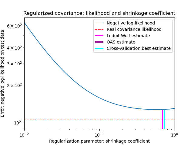
Компромисс смещения и дисперсии при установке усадки: сравнение вариантов оценок Ледуа-Вольфа и OAS
Рекомендации
Чен и др., «Алгоритмы сжатия для оценки ковариации MMSE», IEEE Trans. на знак. Proc., Volume 58, Issue 10, October 2010.
Примеры
- См. В разделе Оценка ковариации усадки: LedoitWolf против OAS и максимальное правдоподобие пример того, как подогнать
OASобъект к данным. - См. Оценку Ледуа-Вольфа и OAS для визуализации разницы среднеквадратических ошибок между a
LedoitWolfиOASоценкой ковариации.
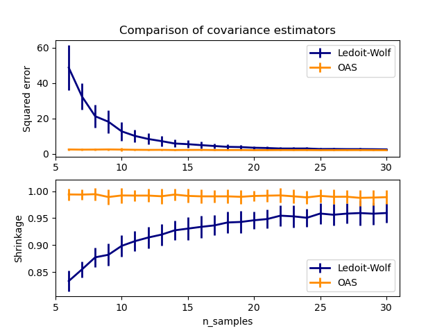
2.6.3. Редкая обратная ковариация
Матрица, обратная ковариационной матрице, часто называемая матрицей точности, пропорциональна матрице частичной корреляции. Это дает частичную независимость отношениям. Другими словами, если два признака независимы друг от друга условно, соответствующий коэффициент в матрице точности будет равен нулю. Вот почему имеет смысл оценивать матрицу разреженной точности: оценка ковариационной матрицы лучше обусловлена изучением отношений независимости от данных. Это называется ковариационным отбором .
В ситуации с малой выборкой, в которой n_samples порядок n_features или меньше, разреженные оценки обратной ковариации, как правило, работают лучше, чем оценки сжатой ковариации. Однако в противоположной ситуации или для сильно коррелированных данных они могут быть численно нестабильными. Кроме того, в отличие от оценщиков усадки, разреженные оценщики могут восстанавливать недиагональную структуру.
Оценщик GraphicalLasso использует l1 штраф для обеспечения разреженности на высокоточной матрице: тем выше его alpha параметр, тем более разреженной прецизионную матрицу. Соответствующий GraphicalLassoCV объект использует перекрестную проверку для автоматической установки alpha параметра.
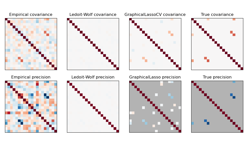
Сравнение максимального правдоподобия, усадки и разреженных оценок ковариации и матрицы точности в настройках очень малых выборок.
Примечание Восстановление структуры
Восстановление графической структуры из корреляций в данных — непростая задача. Если вы заинтересованы в таком восстановлении, имейте в виду, что:
- Восстановление легче из корреляционной матрицы, чем из ковариационной матрицы: стандартизируйте свои наблюдения перед запуском
GraphicalLasso - Если в нижележащем графе есть узлы с гораздо большим количеством соединений, чем в среднем узле, алгоритм пропустит некоторые из этих соединений.
- Если количество ваших наблюдений невелико по сравнению с количеством ребер в вашем нижележащем графе, вы не сможете его восстановить.
- Даже если вы находитесь в благоприятных условиях восстановления, альфа-параметр, выбранный путем перекрестной проверки (например, с использованием
GraphicalLassoCVобъекта), приведет к выбору слишком большого количества ребер. Однако соответствующие ребра будут иметь больший вес, чем нерелевантные.
Математическая формулировка следующая:
$$hat{K} = mathrm{argmin}_K big( mathrm{tr} S K — mathrm{log} mathrm{det} K + alpha |K|_1 big)$$
Где $K$ — матрица точности, которую необходимо оценить, и $S$ — это выборочная ковариационная матрица. $|K|_1$ — сумма модулей недиагональных коэффициентов $K$. Для решения этой проблемы используется алгоритм GLasso из статьи Friedman 2008 Biostatistics. Это тот же алгоритм, что и в glasso пакете R.
Примеры
- Оценка разреженной обратной ковариации: пример синтетических данных, показывающих восстановление структуры и сравнение с другими оценками ковариации.
- Визуализация структуры фондового рынка: пример реальных данных фондового рынка, определение наиболее связанных символов.
Рекомендации
- Фридман и др., «Оценка разреженной обратной ковариации с помощью графического лассо» , Biostatistics 9, стр. 432, 2008 г.
2.6.4. Оценка робастной ковариации
Реальные наборы данных часто подвержены ошибкам измерения или записи. Регулярные, но необычные наблюдения также могут появляться по разным причинам. Наблюдения, которые случаются очень редко, называются выбросами. Эмпирическая оценка ковариации и сжатая оценка ковариации, представленные выше, очень чувствительны к наличию выбросов в данных. Следовательно, следует использовать надежные оценщики ковариации для оценки ковариации реальных наборов данных. В качестве альтернативы можно использовать робастные оценщики ковариации для обнаружения выбросов и отбрасывания / уменьшения веса некоторых наблюдений в соответствии с дальнейшей обработкой данных.
В sklearn.covariance пакете реализована надежная оценка ковариации, определитель минимальной ковариации 3 .
2.6.4.1. Определитель минимальной ковариации
Оценщик, определяющий минимальную ковариацию, — это надежный оценщик ковариации набора данных, представленный PJ Rousseeuw в 3 . Идея состоит в том, чтобы найти заданную пропорцию (h) «хороших» наблюдений, которые не являются выбросами, и вычислить их эмпирическую ковариационную матрицу. Эта эмпирическая ковариационная матрица затем масштабируется, чтобы компенсировать выполненный выбор наблюдений («этап согласованности»). Вычислив оценку определителя минимальной ковариации, можно присвоить веса наблюдениям в соответствии с их расстоянием Махаланобиса, что приведет к повторной оценке ковариационной матрицы набора данных («этап повторного взвешивания»).
Rousseeuw и Van Driessen 4 разработали алгоритм FastMCD для вычисления определителя минимальной ковариации. Этот алгоритм используется в scikit-learn при подгонке объекта MCD к данным. Алгоритм FastMCD также одновременно вычисляет надежную оценку местоположения набора данных.
Сырые оценки могут быть доступны как raw_location_ и raw_covariance_ атрибутами из MinCovDet надежного объекта ковариационной оценивани.
Рекомендации
- 3 PJ Rousseeuw. Наименьшая медиана квадратов регрессии. Дж. Ам Стат Асс, 79: 871, 1984.
- 4 Быстрый алгоритм для определения определителя минимальной ковариации, 1999, Американская статистическая ассоциация и Американское общество качества, TECHNOMETRICS.
Примеры
- См. Пример надежной и эмпирической ковариационной оценки, чтобы узнать, как подогнать
MinCovDetобъект к данным, и посмотрите, насколько оценка остается точной, несмотря на наличие выбросов. - См оценку ковариационной Robust и Махаланобиса расстояния Актуальность визуализировать разницу между
EmpiricalCovarianceиMinCovDetковариации оценок с точки зрения расстояния Махаланобиса (так мы получим более точную оценку точности матрицы тоже).
Авторы
Гай Е.В.
Организация
ГНЦ РФ – Физико-энергетический институт имени А.И. Лейпунского, Обнинск, Россия
Аннотация
Обработка экспериментальных данных методами математической статистики позволяет оценить лежащие в их основе физические закономерности или, по крайней мере, построить непрерывную аппроксиманту этих данных. Обычно при такой обработке используются декларированные статистические и систематические погрешности экспериментальных данных. В классической математической статистике проверка согласованности этих погрешностей с наблюдаемым разбросом данных осуществляется с помощью критерия χ2. В настоящей работе показано, что при большом числе экспериментальных точек погрешность оценки определяется систематическими погрешностями этих точек, но значение критерия χ2 от них не зависит и поэтому он не замечает несоответствия между их декларирированными и наблюдаемыми значениями.
Ключевые слова
критерий χ2, погрешности, МНК, функция правдоподобия, дисперсия экспериментальных данных, систематические ошибки
Полная версия статьи (PDF, 3996 кб)
Список литературы
УДК 539.17
Вопросы атомной науки и техники. Cер. Ядерные константы, 2011-2012, вып. 1-2, c. 8-26
Фильтр Калмана — это легко
Время на прочтение
18 мин
Количество просмотров 56K

Много людей, в первый раз сталкивающихся в работе с датчиками, склонны считать, что получаемые показания — это точные значения. Некоторые вспоминают, что в показаниях всегда есть погрешности и ошибки. Чтобы ошибки в измерениях не приводили к ошибкам в функционировании системы в целом, данные датчиков необходимо обрабатывать. На ум сразу приходит словосочетание “фильтр Калмана”. Но слава этого “страшного” алгоритма, малопонятные формулы и разнообразие используемых обозначений отпугивают разработчиков. Постараемся разобраться с ним на практическом примере.
Об алгоритме
Что же нам потребуется для работы фильтра Калмана?
- Нам потребуется модель системы.
- Модель должна быть линейной (об этом чуть позже).
- Нужно будет выбрать переменные, которые будут описывать состояние системы (“вектор состояния”).
- Мы будем производить измерения и вычисления в дискретные моменты времени (например, 10 раз в секунду). Нам потребуется модель наблюдения.
- Для работы фильтра достаточно данных измерений в текущий момент времени и результатов вычислений с предыдущего момента времени.
Алгоритм работает итеративно. На каждом шаге алгоритм берёт данные датчиков (с шумом и другими проблемами), вектор состояния с предыдущего шага и по этим данным оценивает состояние системы на текущем шаге. Кроме того, он еще отслеживает насколько мы можем быть уверены, что наш текущий вектор состояний соответствует истинному положению дел (разброс значений для каждой переменной в векторе).
Обычно используются следующие обозначения:
 — вектор состояния;
 — мера неопределенности вектора состояния. Представляет из себя ковариационную матрицу (об этом позже — это будет, наверное, самая сложная часть).
Содержимое вектора состояния зависит от фантазии разработчика и решаемой задачи. Например, мы можем отслеживать координаты объекта, а также его скорость и ускорение. В этом случае получается вектор из трёх переменных: {позиция, скорость, ускорение} (для одномерного случая; для 3D мира будет по одному такому набору для каждой оси, то есть, 9 значений в векторе)
По сути, речь идёт о совместном распределении случайных величин
В фильтре Калмана мы предполагаем, что все погрешности и ошибки (как во входных данных, так и в оценке вектора состояния) имеют нормальное распределение. А для многомерного нормального распределения его полностью определяют два параметра: математическое ожидание вектора и его ковариационная матрица.
Математическая модель системы / процесса
Мы имеем дело с динамической системой, т.е. состояние системы меняется со временем. Имея модель системы, фильтр Калмана может предугадывать, каким будет состояние системы в следующий момент времени. Именно это позволяет фильтру так эффективно устранять шум и оценивать параметры, которые не наблюдаются (не измеряются) напрямую.
Фильтр Калмана накладывает ограничения на используемые модели: это должны быть дискретные модели в пространстве состояний. А ещё они должны быть линейными.
Дискретные и линейные?
Дискретность означает для нас то, что модель работает “шагами”. На каждом шаге мы вычисляем новое состояние системы по вектору состояния с предыдущего шага. Обычно, модели такого рода задаются системой разностных уравнений.
По поводу линейности: каждое уравнение системы является линейным уравнением, задающим новое значение переменной состояния. Т.е. никаких косинусов, синусов, возведений в степень и даже сложений с константой.
Такую модель удобно представлять в виде разностного матричного уравнения:

Давайте разберём это уравнение подробно. В первую очередь, нас интересует первое слагаемое ( ) — это как раз модель эволюции процесса. А матрица
  (также встречаются обозначения
  ,
,  ) — называется матрицей процесса (state transition matrix). Она задаёт систему линейных уравнений, описывающих, как получается новое состояние системы из предыдущего.
Например, для равноускоренного движения матрица будет выглядеть так:

Первая строка матрицы — хорошо знакомое уравнение  . Аналогично, вторая строка матрицы описывает изменение скорости. Третья строка описывает изменение ускорения.
А что же с остальными слагаемыми?
В некоторых случаях, мы напрямую управляем процессом (например, управляем квадракоптером с помощью пульта Д/У) и нам достоверно известны задаваемые параметры (заданная на пульте скорость полёта). Второе слагаемое — это модель управления. Матрица  называется матрицей управления, а вектор
  — вектор управляющих воздействий. В случаях когда мы только наблюдаем за процессом, это слагаемое отсутствует.
Последнее слагаемое —  — это вектор ошибки модели. Модель равноускоренного движения абсолютно точно описывает положение объекта. Однако в реальном мире есть множество случайных факторов — дороги неровные, дует ветер, и т.п. Иногда, процесс сложен и приходится использовать упрощённую модель, которая не учитывает все аспекты. Именно так возникает ошибка модели.
То, что мы записываем это слагаемое, не означает, что мы знаем ошибку на каждом шаге или описываем её аналитически. Однако фильтр Калмана делает важное предположение — ошибка имеет нормальное распределение с нулевым математическим ожиданием и ковариационной матрицей  . Эта матрица очень важна для стабильной работы фильтра и мы её рассмотрим позже.
Модель наблюдения
Не всегда получается так, что мы измеряем интересующие нас параметры напрямую (например, мы измеряем скорость вращения колеса, хотя нас интересует скорость автомобиля). Модель наблюдения описывает связь между переменными состояния и измеряемыми величинами:

 — это вектор измерения/наблюдения.Это значения, получаемые с датчиков системы.
Первое слагаемое  — модель, связывающая вектор состояния с соответствующими ему показаниями датчиков. (Такой выбор модели может показаться странным, ведь наша задача — получить из , а эта модель получает из . Но это действительно так. В частности, это необходимо потому, что некоторые переменные состояния из могут отсутствовать в ).
Второе слагаемое  — это вектор ошибок измерения. Как и в случае с предыдущими ошибками, предполагается, что она имеет нормальное распределение с нулевым математическим ожиданием.
  — ковариационная матрица, соответствующая вектору .
Вернёмся к нашему примеру. Пусть у нас на роботе установлен один единственный датчик — GPS приёмник (“измеряет” положение). В этом случае матрица  будет выглядеть следующим образом:

Строки матрицы соответствуют переменным в векторе состояния, столбцы — элементам вектора измерений. В первой строке матрицы находится значение “1” так как единица измерения положения в векторе состояния совпадает с единицей измерения значения в векторе измерений. Остальные строки содержат “0” потому что переменные состояния соответствующие этим строкам не измеряются датчиком.
Что будет, если датчик и модель используют разные единицы измерения? А если датчиков несколько?
Например, модель использует метры, а датчик — количество оборотов колеса. В этом случае матрица будет выглядеть так:

Количество датчиков ничем (кроме здравого смысла) не ограничено.
Например, добавим спидометр:

Второй столбец матрицы соответствует нашему новому датчику.
Несколько датчиков могут измерять один и тот же параметр. Добавим ещё один датчик скорости:

Ковариационные матрицы и где они обитают
Для настройки фильтра нам потребуется заполнить несколько ковариационных матриц:
, и .
Ковариационные матрицы?
Для нормально распределенной случайной величины её математическое ожидание и дисперсия полностью определяют её распределение. Дисперсия — это мера разброса случайной величины. Чем больше дисперсия — тем сильнее может отклоняться случайная величина от её математического ожидания. Ковариационная матрица — это многомерный аналог дисперсии, для случая, когда у нас не одна случайная величина, а случайный вектор.
В одной статье сложно уместить всю теорию вероятностей, поэтому ограничимся сугубо практическими свойствами ковариационных матриц. Это симметричные квадратные матрицы, на главной диагонали которой располагаются дисперсии элементов вектора. Остальные элементы матрицы — ковариации между компонентами вектора. Ковариация показывает, насколько переменные зависят друг от друга.
Проиллюстрируем влияние мат. ожидания, дисперсии и ковариации.
Начнём с одномерного случая. Функция плотности вероятности нормального распределения — знаменитая колоколообразная кривая. Горизонтальная ось — значение случайной величины, а вертикальная ось — сравнительная вероятность того что случайная величина примет это значение:

Чем меньше дисперсия — тем меньше ширина колокола.
Понятие ковариации возникает для совместного распределения нескольких случайных величин. Когда случайные величины независимы, то ковариация равна нулю:

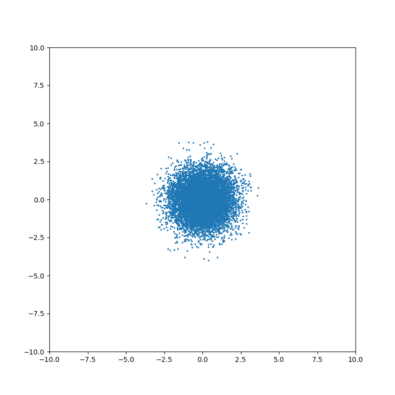
Ненулевое значение ковариации означает, что существует связь между значениями случайных величин:

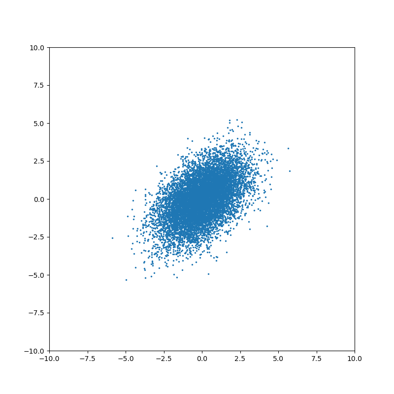

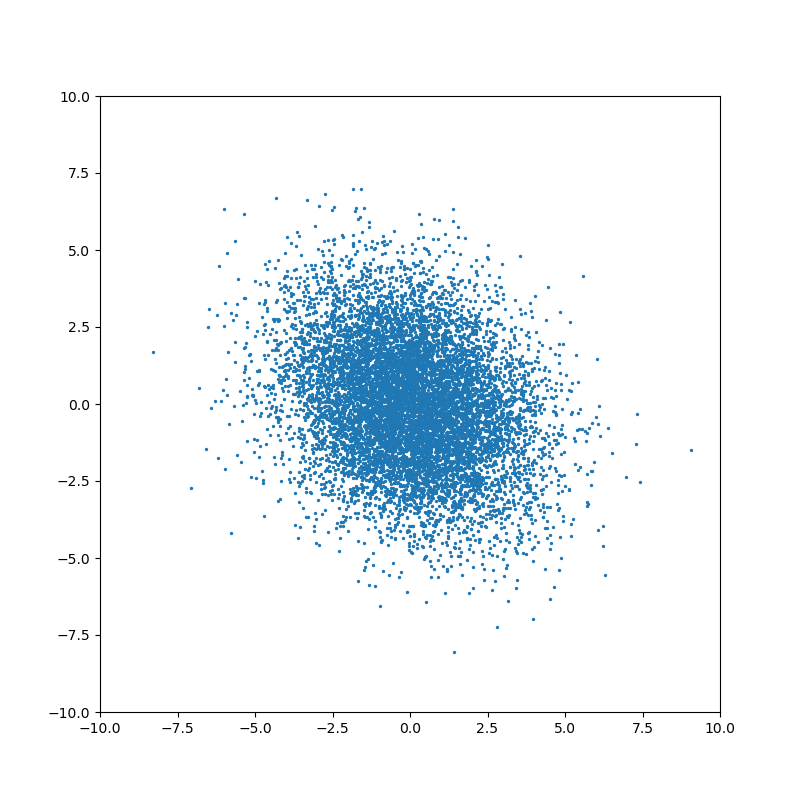
На каждом шаге фильтр Калмана строит предположение о состоянии системы, исходя из предыдущей оценки состояния и данных измерений. Если неопределенности вектора состояния выше, чем ошибка измерения, то фильтр будет выбирать значения ближе к данным измерений. Если ошибка измерения больше оценки неопределенности состояния, то фильтр будет больше “доверять” данным моделирования. Именно поэтому важно правильно подобрать значения ковариационных матриц — основного инструмента настройки фильтра.
Рассмотрим каждую матрицу подробнее:
— ковариационная матрица состояния
Квадратная матрица, порядок матрицы равен размеру вектора состояния
Как уже было сказано выше, эта матрица определяет “уверенность” фильтра в оценке переменных состояния. Алгоритм самостоятельно обновляет эту матрицу в процессе работы. Однако нам нужно установить начальное состояние, вместе с исходным предположением о векторе состояния.
Во многих случаях нам неизвестны значения ковариации между переменными для изначального состояния (элементы матрицы, расположенные вне главной диагонали). Поэтому можно проигнорировать их, установив равными 0. Фильтр самостоятельно обновит значения в процессе работы. Если же значения ковариации известны, то, конечно же, стоит использовать их.
Дисперсию же проигнорировать не выйдет. Необходимо установить значения дисперсии в зависимости от нашей уверенности в исходном векторе состояния. Для этого можно воспользоваться правилом трёх сигм: значение случайной величины попадает в диапазон  с вероятностью 99.7%.
Пример
Допустим, нам нужно установить дисперсию для переменной состояния — скорости робота. Мы знаем что максимальная скорость передвижения робота — 10 м/с. Но начальное значение скорости нам неизвестно. Поэтому, мы выберем изначальное значение переменной — 0 м/с, а среднеквадратичное отклонение  ;
;  Соответственно, дисперсия
  .
.
— ковариационная матрица шума измерений
Квадратная матрица, порядок матрицы равен размеру вектора наблюдения (количеству измеряемых параметров).
Во многих случаях можно считать, что измерения не коррелируют друг с другом. В этом случае матрица будет являться диагональной матрицей, где все элементы вне главной диагонали равны нулю. Достаточно будет установить значения дисперсии для каждого измеряемого параметра. Иногда эти данные можно найти в документации к используемым датчика. Однако, если справочной информации нет, то можно оценить дисперсию, измеряя датчиком заранее известное эталонное значение, или воспользоваться правилом трёх сигм.
— ковариационная матрица ошибки модели
Квадратная матрица, порядок матрицы равен размеру вектора состояния.
С этой матрицей обычно возникает наибольшее количество вопросов. Что означает ошибка модели? Каков смысл этой матрицы и за что она отвечает? Как заполнять эту матрицу? Рассмотрим всё по порядку.
Каждый раз, когда фильтр предсказывает состояние системы, используя модель процесса, он увеличивает неуверенность в оценке вектора состояния. Для одномерного случая формула выглядит приблизительно следующим образом:

Если установить очень маленькое значение , то этап предсказания будет слабо увеличивать неопределенность оценки. Это означает, что мы считаем, что наша модель точно описывает процесс.
Если же установить большое значение , то этап предсказания будет сильно увеличивать неопределенность оценки. Таким образом, мы показываем что модель может содержать неточности или неучтенные факторы.
Для многомерного случая формула выглядит несколько сложнее, но смысл схожий. Однако, есть важное отличие: эта матрица указывает, на какие переменные состояния будут в первую очередь влиять ошибки модели и неучтённые факторы.
Допустим, мы отслеживаем перемещение робота, используя модель равноускоренного движения, и вектор состояния содержит следующие переменные: положение x, скорость v и ускорение a. Однако, наша модель не учитывает, что на дороге встречаются неровности.
Когда робот проходит неровность, показания датчиков и предсказание модели начнут расходиться. Структура матрицы будет определять, как фильтр отреагирует на это расхождение.
Мы можем выдвинуть различные предположения относительно природы шума. Для нашего примера с равноускоренным движением логично было бы предположить, что неучтённые факторы (неровность дороги) в первую очередь влияют на ускорение. Этот подход применим ко многим структурам модели, где в векторе состояния присутствует переменная и несколько её производных по времени (например, положение и производные: скорость и ускорение). Матрица выбирается таким образом, чтобы наибольшее значение соответствовало самому высокому порядку производной.
Так как же заполняется матрица Q?
Обычно используют модель-приближение. Рассмотрим на примере модели равноускоренного движения:
Модель непрерывного белого шума
Мы предполагаем, что ускорение постоянно на каждом шаге. Но из-за неровностей дороги ускорение, на самом деле, постоянно изменяется. Мы можем предположить, что изменение ускорения происходит под воздействием непрерывного белого шума с нулевым математическим ожиданием (т.е. усреднив все небольшие изменения ускорения за время движения робота мы получаем 0)
В этой модели матрица Q рассчитывается следующим образом

Мы формируем матрицу Qc в соответствии со структурой вектора состояния. Наивысшему порядку производной соответствует правый нижний элемент матрицы. В случае, если в векторе состояния несколько таких переменных, то каждая из них учитывается в матрице.
Для нашей модели равноускоренного движения матрица будет выглядеть так:

 — спектральная плотность мощности белого шума
Подставляем матрицу процесса, соответствующую нашей модели:

После перемножения и интегрирования получаем:

Модель “кусочного” белого шума
Мы предполагаем, что ускорение на самом деле постоянно в течение каждого шага моделирования, но дискретно и независимо меняется между шагами. Выглядит очень похоже на предыдущую модель, но небольшая разница есть

 — мощность шума
 — наивысший порядок производной, используемой в модели (т.е. ускорение для вышеописанной модели)
В этой модели матрица определяется следующим образом:
![$ Q = mathbb{E}[,Gammaomega(t)omega(t)Gamma^T],=Gammasigma_upsilon^2Gamma^T $](https://habrastorage.org/getpro/habr/formulas/68f/0bb/a32/68f0bba3267049b97faff063484e96eb.svg)
Из матрицы процесса F
берём столбец с наивысшим порядком производной

и подставляем в формулу. В итоге получаем:

Обе модели являются приближениями того, что происходит на самом деле в реальности. На практике, приходится экспериментировать и выяснять, какая модель подходит лучше в каждом отдельном случае. Плюсом второй модели является то, что мы оперируем дисперсией шума, с которой уже хорошо умеем работать.
Простейший подход
В некоторых случаях прибегают к грубому упрощению: устанавливают все элементы матрицы равными нулю, за исключением элементов, соответствующих максимальным порядкам производных переменных состояния.
Действительно, если рассчитать по одному из приведённых выше методов, при достаточно малых значениях  , значения элементов матрицы оказываются очень близкими к нулю.
Т.е. для нашей модели равноускоренного движения можно взять матрицу следующего вида:

И хотя такой подход не совсем корректен, его можно использовать в качестве первого приближения или для экспериментов. Без сомнения, не стоит выбирать матрицу таким образом для любых важных задач без весомых причин.
Важное замечание
Во всех примерах выше используется вектор состояния  и может показаться, что во всех случаях дисперсия, соответствующая наивысшему порядок производной, находится в правом нижнем углу матрицы. Это не так.
Рассмотрим вектор состояния 
Матрица будет представлять собой блочную матрицу, где отдельные блоки 3х3 элементов будут соответствовать группам и  . Остальные элементы матрицы будут равны нулю.
Дисперсия, соответствующая наивысшим порядкам производных  и
и  , будет находиться на 3-ей и 5-ой позициях на главной диагонали матрицы.
Однако, на практике нет никакого смысла перемешивать порядок переменных состояния таким образом, чтобы порядки производных шли не по очереди — это просто неудобно.
Пример кода
Нет смысла изобретать велосипед и писать свою собственную реализацию фильтра Калмана, когда существует множество готовых библиотек. Я выбрал язык python и библиотеку filterpy для примера.
Чтобы не загромождать пример, возьмем одномерный случай. Одномерный робот оборудован одномерным GPS, который определяет положение с некоторой погрешностью.
Моделирование данных датчиков
Начнём с равномерного движения:
Simulator.py
import numpy as np
import numpy.random

# Моделирование данных датчика
def simulateSensor(samplesCount, noiseSigma, dt):
   # Шум с нормальным распределением. мат. ожидание = 0, среднеквадратичное отклонение = noiseSigma
   noise = numpy.random.normal(loc = 0.0, scale = noiseSigma, size = samplesCount)

   trajectory = np.zeros((3, samplesCount))

   position = 0
   velocity = 1.0
   acceleration = 0.0

   for i in range(1, samplesCount):
       position = position + velocity * dt + (acceleration * dt ** 2) / 2.0
       velocity = velocity + acceleration * dt
       acceleration = acceleration

       trajectory[0][i] = position
       trajectory[1][i] = velocity
       trajectory[2][i] = acceleration

   measurement = trajectory[0] + noise

   return trajectory, measurement # Истинное значение и данные "датчика" с шумом
Визуализируем результаты моделирования:
Код
import matplotlib.pyplot as plt
dt = 0.01
measurementSigma = 0.5
trajectory, measurement = simulateSensor(1000, measurementSigma, dt)

plt.title("Данные датчика")
plt.plot(measurement, label="Измерение", color="#99AAFF")
plt.plot(trajectory[0], label="Истинное значение", color="#FF6633")
plt.legend()
plt.show()
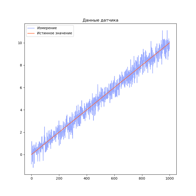
Реализация фильтра
Для начала выберем модель системы. Я решил взять 3 переменных состояния: положение, скорость и ускорение. В качестве модели процесса возьмем модель равноускоренного движения:
У нас единственный датчик, который напрямую измеряет положение. Поэтому модель наблюдения получается очень простой:

Мы предполагаем, что наш робот находится в точке 0 и имеет нулевые скорость и ускорение в начальный момент времени:

Однако, мы не уверены, что это именно так. Поэтому установим матрицу ковариации для начального состояния с большими значениями на главной диагонали:

Я воспользовался функцией библиотеки filterpy для расчёта ковариационной матрицы ошибки модели: filterpy.common.Q_discrete_white_noise. Эта функция использует модель непрерывного белого шума.
Код
import filterpy.kalman
import filterpy.common
import matplotlib.pyplot as plt
import numpy as np
import numpy.random
from Simulator import simulateSensor # моделирование датчиков

dt = 0.01                       # Шаг времени
measurementSigma = 0.5          # Среднеквадратичное отклонение датчика
processNoise = 1e-4             # Погрешность модели

# Моделирование данных датчиков
trajectory, measurement = simulateSensor(1000, measurementSigma, dt)

# Создаём объект KalmanFilter
filter = filterpy.kalman.KalmanFilter(dim_x=3,      # Размер вектора стостояния
                                     dim_z=1)      # Размер вектора измерений

# F - матрица процесса - размер dim_x на dim_x - 3х3
filter.F = np.array([ [1,   dt,     (dt**2)/2],
                     [0,   1.0,    dt],
                     [0,   0,      1.0]])


# Матрица наблюдения - dim_z на dim_x - 1x3
filter.H = np.array([[1.0, 0.0, 0.0]])

# Ковариационная матрица ошибки модели
filter.Q = filterpy.common.Q_discrete_white_noise(dim=3, dt=dt, var=processNoiseVariance)

# Ковариационная матрица ошибки измерения - 1х1
filter.R = np.array([[measurementSigma*measurementSigma]])

# Начальное состояние.
filter.x = np.array([0.0, 0.0, 0.0])

# Ковариационная матрица для начального состояния
filter.P = np.array([[10.0, 0.0,  0.0],
                    [0.0,  10.0, 0.0],
                    [0.0,  0.0,  10.0]])

filteredState = []
stateCovarianceHistory = []

# Обработка данных
for i in range(0, len(measurement)):
   z = [ measurement[i] ]                      # Вектор измерений
   filter.predict()                            # Этап предсказания
   filter.update(z)                            # Этап коррекции

   filteredState.append(filter.x)
   stateCovarianceHistory.append(filter.P)

filteredState = np.array(filteredState)
stateCovarianceHistory = np.array(stateCovarianceHistory)

# Визуализация
plt.title("Kalman filter (3rd order)")
plt.plot(measurement, label="Измерение", color="#99AAFF")
plt.plot(trajectory[0], label="Истинное значение", color="#FF6633")
plt.plot(filteredState[:, 0], label="Оценка фильтра", color="#224411")
plt.legend()
plt.show()
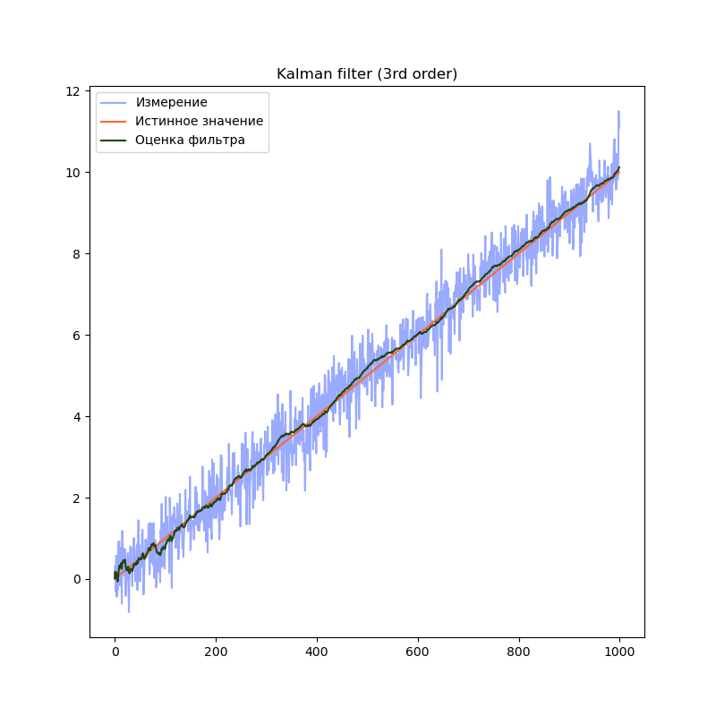
Бонус — сравнение различных порядков моделей
Сравним поведение фильтра с моделями разного порядка. Для начала, смоделируем более сложный сценарий поведения робота. Пусть робот находится в покое первые 20% времени, затем движется равномерно, а затем начинает двигаться равноускоренно:
Simulator.py
# Моделирование данных датчика
def simulateSensor(samplesCount, noiseSigma, dt):
   # Шум с нормальным распределением. мат. ожидание = 0, среднеквадратичное отклонение = noiseSigma
   noise = numpy.random.normal(loc = 0.0, scale = noiseSigma, size = samplesCount)

   trajectory = np.zeros((3, samplesCount))

   position = 0
   velocity = 0.0
   acceleration = 0.0

   for i in range(1, samplesCount):
       position = position + velocity * dt + (acceleration * dt ** 2) / 2.0
       velocity = velocity + acceleration * dt
       acceleration = acceleration

       # Переход на равномерное движение
       if(i == (int)(samplesCount * 0.2)):
           velocity = 10.0

       # Переход на равноускоренное движение
       if (i == (int)(samplesCount * 0.6)):
           acceleration = 10.0

       trajectory[0][i] = position
       trajectory[1][i] = velocity
       trajectory[2][i] = acceleration

   measurement = trajectory[0] + noise

   return trajectory, measurement # Истинное значение и данные "датчика" с шумом
В предыдущем примере мы использовали модель, содержащую переменную (положение) и две производных её по времени (скорость и ускорение). Посмотрим, что будет, если избавиться от одной или обеих производных:
2-й порядок
# Создаём объект KalmanFilter
filter = filterpy.kalman.KalmanFilter(dim_x=2,      # Размер вектора стостояния
                                     dim_z=1)      # Размер вектора измерений

# F - матрица процесса - размер dim_x на dim_x - 2х2
filter.F = np.array([ [1,   dt],
                     [0,   1.0]])


# Матрица наблюдения - dim_z на dim_x - 1x2
filter.H = np.array([[1.0, 0.0]])

filter.Q = [[dt**2,       dt],
           [   dt,      1.0]] * processNoise

# Начальное состояние.
filter.x = np.array([0.0, 0.0])

# Ковариационная матрица для начального состояния
filter.P = np.array([[8.0, 0.0],
                    [0.0, 8.0]])
1-й порядок
# Создаём объект KalmanFilter
filter = filterpy.kalman.KalmanFilter(dim_x=1,      # Размер вектора стостояния
                                     dim_z=1)      # Размер вектора измерений

# F - матрица процесса - размер dim_x на dim_x - 1х1
filter.F = np.array([ [1.0]])


# Матрица наблюдения - dim_z на dim_x - 1x1
filter.H = np.array([[1.0]])

# Ковариационная матрица ошибки модели
filter.Q = processNoise

# Ковариационная матрица ошибки измерения - 1х1
filter.R = np.array([[measurementSigma*measurementSigma]])

# Начальное состояние.
filter.x = np.array([0.0])

# Ковариационная матрица для начального состояния
filter.P = np.array([[8.0]])
Сравним результаты:
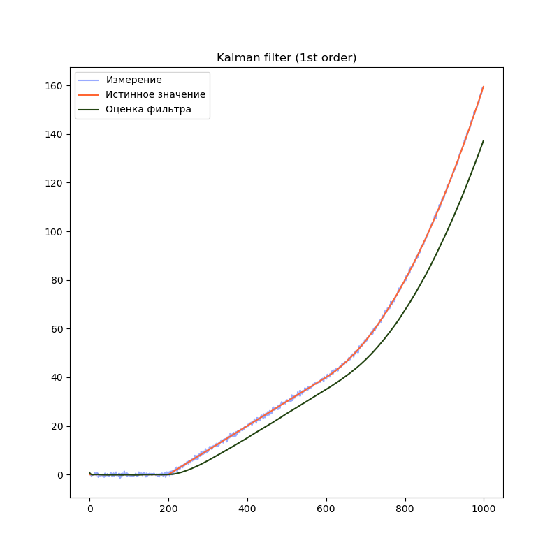
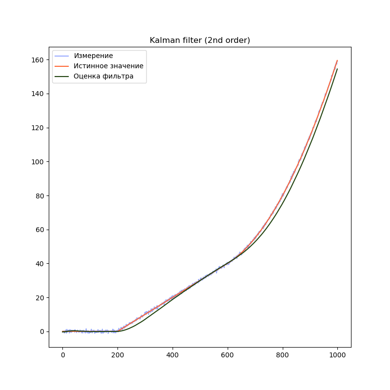

На графиках сразу заметно, что модель первого порядка начинает отставать от истинного значения на участках равномерного движения и равноускоренного движения. Модель второго порядка успешно справляется с участком равномерного движения, но так же начинает отставать на участке равноускоренного движения. Модель третьего порядка справляется со всеми тремя участками.
Однако, это не означает что нужно использовать модели высокого порядка во всех случаях. В нашем примере, модель третьего порядка справляется с участком равномерного движения несколько хуже модели второго порядка, т.к. фильтр интерпретирует шум сенсора как изменение ускорения. Это приводит к колебанию оценки фильтра. Стоит подбирать порядок модели в соответствии с планируемыми режимами работы фильтра.
Нелинейные модели и фильтр Калмана
Почему фильтр Калмана не работает для нелинейных моделей и что делать
Всё дело в нормальном распределении. При применении линейных преобразованийк нормально распределенной случайной величине, результирующее распределение будет представлять собой нормальное распределение, или будет пропорциональным нормальному распределению. Именно на этом принципе и строится математика фильтра Калмана.
Есть несколько модификаций алгоритма, которые позволяют работать с нелинейными моделями.
Например:
Extended Kalman Filter (EKF) — расширенный фильтр Калмана. Этот подход строит линейное приближение модели на каждом шаге. Для этого требуется рассчитать матрицу вторых частных производных функции модели, что бывает весьма непросто. В некоторых случаях, аналитическое решение найти сложно или невозможно, и поэтому используют численные методы.
Unscented Kalman Filter (UKF). Этот подход строит приближение распределения получающегося после нелинейного преобразования при помощи сигма-точек. Преимуществом этого метода является то, что он не требует вычисления производных.
Мы рассмотрим именно Unscented Kalman Filter
Unscented Kalman Filter и почему он без запаха
Основная магия этого алгоритма заключается в методе, который строит приближение распределения плотности вероятности случайной величины после прохождения через нелинейное преобразование. Этот метод называется unscented transform — сложнопереводимое на русский язык название. Автор этого метода, Джеффри Ульман, не хотел, чтобы его разработку называли “Фильтр Ульмана”. Согласно интервью, он решил назвать так свой метод после того как увидел дезодорант без запаха (“unscented deodorant”) на столе в лаборатории, где он работал.
Этот метод достаточно точно строит приближение функции распределения случайной величины, но что более важно — он очень простой.
Для использования UKF не придётся реализовывать какие-либо дополнительные вычисления, за исключением моделей системы. В общем виде, нелинейная модель не может быть представлена в виде матрицы, поэтому мы заменяем матрицы и на функции  и
и  . Однако смысл этих моделей остаётся тем же.
Реализуем unscented Kalman filter для линейной модели из прошлого примера:
Код
import filterpy.kalman
import filterpy.common
import matplotlib.pyplot as plt
import numpy as np
import numpy.random
from Simulator import simulateSensor, CovarianceQ

dt = 0.01
measurementSigma = 0.5
processNoiseVariance = 1e-4

# Функция наблюдения - аналог матрицы наблюдения
# Преобразует вектор состояния x в вектор измерений z
def measurementFunction(x):
   return np.array([x[0]])

# Функция процесса - аналог матрицы процесса
def stateTransitionFunction(x, dt):
   newState = np.zeros(3)
   newState[0] = x[0] + dt * x[1] + ( (dt**2)/2 ) * x[2]
   newState[1] = x[1] + dt * x[2]
   newState[2] = x[2]

   return newState


trajectory, measurement = simulateSensor(1000, measurementSigma)

# Для unscented kalman filter необходимо выбрать алгоритм выбора сигма-точек
points = filterpy.kalman.JulierSigmaPoints(3, kappa=0)

# Создаём объект UnscentedKalmanFilter
filter = filterpy.kalman.UnscentedKalmanFilter(dim_x = 3,
                                              dim_z = 1,
                                              dt = dt,
                                              hx = measurementFunction,
                                              fx = stateTransitionFunction,
                                              points = points)


# Ковариационная матрица ошибки модели
filter.Q = filterpy.common.Q_discrete_white_noise(dim=3, dt=dt, var=processNoiseVariance)

# Ковариационная матрица ошибки измерения - 1х1
filter.R = np.array([[measurementSigma*measurementSigma]])

# Начальное состояние.
filter.x = np.array([0.0, 0.0, 0.0])

# Ковариационная матрица для начального состояния
filter.P = np.array([[10.0, 0.0,  0.0],
                    [0.0,  10.0, 0.0],
                    [0.0,  0.0,  10.0]])

filteredState = []
stateCovarianceHistory = []

for i in range(0, len(measurement)):
   z = [ measurement[i] ]
   filter.predict()
   filter.update(z)

   filteredState.append(filter.x)
   stateCovarianceHistory.append(filter.P)

filteredState = np.array(filteredState)
stateCovarianceHistory = np.array(stateCovarianceHistory)

plt.title("Unscented Kalman filter")
plt.plot(measurement, label="Измерение", color="#99AAFF")
plt.plot(trajectory[0], label="Истинное значение", color="#FF6633")
plt.plot(filteredState[:, 0], label="Оценка фильтра", color="#224411")
plt.legend()
plt.show()
Разница в коде минимальна. Мы заменили матрицы F и H на функции f(x) и h(x). Это позволяет использовать нелинейные модели системы и/или наблюдения:
# Функция наблюдения - аналог матрицы наблюдения
# Преобразует вектор состояния x в вектор измерений z
def measurementFunction(x):
   return np.array([x[0]])

# Функция процесса - аналог матрицы процесса
def stateTransitionFunction(x, dt):
   newState = np.zeros(3)
   newState[0] = x[0] + dt * x[1] + ( (dt**2)/2 ) * x[2]
   newState[1] = x[1] + dt * x[2]
   newState[2] = x[2]

   return newState
Также, появилась строчка, устанавливающая алгоритм генерации сигма-точек
points = filterpy.kalman.JulierSigmaPoints(3, kappa=0)
Этот алгоритм определяет точность оценки распределения вероятности при прохождении через нелинейное преобразование. К сожалению, существуют только общие рекомендации относительно генерации сигма-точек. Поэтому для каждой отдельной задачи значения параметров алгоритма подбираются экспериментальным путём.
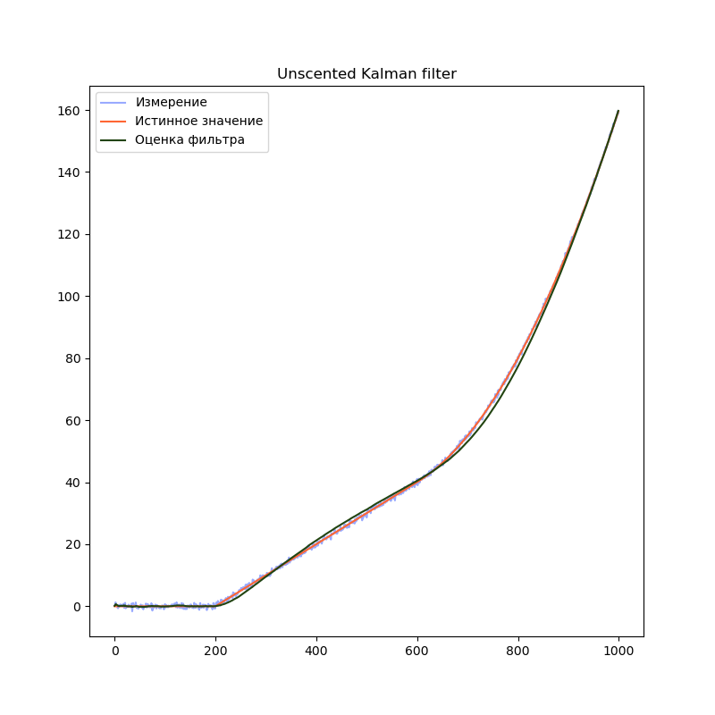
Ожидаемый результат — график оценки положения практически не отличается от обычного фильтра Калмана.
В этом примере используется линейная модель. Однако мы могли бы использовать нелинейные функции. Например, мы могли бы использовать следующую реализацию:
g = 9.8
# Вектор состояния - угол наклона
# Вектор измерений - ускорение вдоль осей X и Y
def measurementFunction(x):
  measurement = np.zeros(2)
  measurement[0] = math.sin(x[0]) * g
  measurement[1] = math.cos(x[0]) * g
  return measurement
Такую модель измерений было бы невозможно использовать в случае с линейным фильтром Калмана
Вместо заключения
За рамками статьи остались теоретические основы фильтра Калмана. Однако объем материала по этой теме ошеломляет. Сложно выбрать хороший источник. Я бы хотел рекомендовать замечательную книгу от автора библиотеки filterpy Roger Labbe (на английском языке). В ней доступно описаны принципы работы алгоритма и сопутствующая теория. Книга представляет собой документ Jupyter notebook, который позволяет в интерактивном режиме экспериментировать с примерами.
Литература
→ Roger Labbe — Kalman and Bayesian Filters in Python
→ Wikipedia